In the previous chapters, we explored how Denoising Score Matching and Diffusion Models can learn to reverse a stochastic (noise-based) process to generate data. These models gradually destroy structure with noise and then learn to painstakingly reverse that process, step by noisy step.
This raises a question: Can we achieve the same goal without noise? What if we could learn a deterministic transformation that smoothly ‘flows’ a simple base distribution (like a Gaussian) into a complex data distribution?
This is the core idea behind Flow Matching. Instead of learning to reverse a noisy, stochastic process, we learn a deterministic vector field of velocities that directly transports probability mass. We saw this ideas earlier in two cases: first with Optimal Transport GANs, where we had to solve a complex and expensive transport matching problem, and then later with (Continuous) Normalizing Flows, which required computing Jacobian determinants in high dimensions. Flow Matching inherits some of these ideas – notably the idea of learning a vector field to move data points from CNFs and the notion of pairing sets of points from Optimal Transport – but avoids many of their computational complexities by making certain approximations. In practice, this approach is often simpler to train, faster to sample from, and offers a different but powerful perspective on generative modeling that those we have looked at so far.
19.1 Learning Objectives
By the end of this notebook, you should have a strong intuition for:
The conceptual difference between stochastic diffusion and deterministic flow matching.
How to define a simple ‘path’ between a noise distribution and a data distribution.
How to train a neural network to predict the ‘velocity’ along this path.
How to generate samples by integrating this learned velocity field using an ODE solver.
Show Code
import numpy as npimport matplotlib.pyplot as pltimport seaborn as snsimport torchfrom torch import nnimport torch.optim as optimfrom matplotlib.animation import FuncAnimationfrom IPython.display import HTMLfrom gen_models_utilities import ( device, create_ring_gaussians, make_loader, load_eth_z_logo_data, make_conditional_loader_onehot, make_conditional_loader_radius, plot_conditional_samples_discrete, plot_conditional_samples_continuous)# Use a consistent styleplt.style.use('seaborn-v0_8-muted')sns.set_context('talk')# for reproducibilitytorch.manual_seed(42)np.random.seed(42)if torch.cuda.is_available(): torch.cuda.manual_seed_all(42)#device = "cpu"print(f'Using device: {device}')
Using device: cuda
19.2 The Noise-Free Limit
As we saw last chapter, Diffusion models work by reversing a stochastic process. The sampling is noisy and requires many steps because it has to undo the randomness that was added during the forward process.
Flow matching takes a more direct route. It learns a deterministic vector field \(v_\theta(x_t, t)\) that defines the velocity of particles as they move from a base distribution \(p_0\) to the target data distribution \(p_1\). The generative process becomes the solution to an ordinary differential equation (ODE):
\[ \frac{dx_t}{dt} = v_\theta(x_t, t) \]
Starting with a sample \(x_0 \sim p_0\), we can find the corresponding data sample \(x_1\) by integrating this equation from \(t=0\) to \(t=1\). The path is smooth and deterministic. This is similar in concept to what we saw in the previous chapter on Continuous Normalizing Flows (CNFs), however, we will see below that they have different training strategies and properties.
19.3 Interpolating a Path
Like with CNFs, we need to define a velocity field \(v_\theta(x_t, t)\) that smoothly transports samples from the base distribution to the data distribution over time. But how should we define the ‘correct’ velocity field to learn? In CNFs, we derived it from the instantaneous change of variables formula, but that required computing Jacobian determinants which can be expensive and required the velocity field to have certain regularity properties so that the integral could be computed efficiently. Moreover, training the velocity field required estimating an integral over the entire flow path, which can be computationally intensive, and the numerical ODE solver used to compute the integral had to be differentiable to allow backpropagation back to the learned velocity field.
In contrast, Flow Matching uses a simple but brilliant trick. We don’t need to simulate a complex forward process (as in Diffusion Models) or estimate some integral of a flow path (as in CNFs). Instead, we just define a synthetic ‘path’ by simply drawing a straight line between a sample from our base distribution and a sample from our data distribution. This pair of samples is often called a synthetic coupling pair.
Let \(x_0 \sim p_\text{base}\) (e.g., a standard Gaussian) and \(x_1 \sim p_\text{data}\) (e.g., our ring of Gaussians). Given these two sampled points, we define an interpolated point \(x_t\) at time \(t \in [0, 1]\) as:
\[ x_t = (1 - t) x_0 + t x_1 \]
This gives us a point on the straight line connecting the noise sample to the data sample. The velocity along this path is constant and easy to calculate:
\[ v_t(x_t) = \frac{dx_t}{dt} = x_1 - x_0 \]
This is our ground truth velocity. For any interpolated point \(x_t\), the target vector is simply the difference vector between the data point and the noise point that created it. This provides a direct, local supervision signal for training our neural network. Another nice benefit of this approach is that it doesn’t place any particular restrictions on the base distribution – it can be Gaussian, uniform, or any other simple distribution from which we can easily sample, since all we need are coupled pairs of points \((x_0, x_1)\) to define our paths. That is, Flow Matching doesn’t require any specific form for \(p_\text{base}\), unlike models such as Diffusion Models that assume (and in fact rely upon) on Gaussian noise to be the final base distribution.
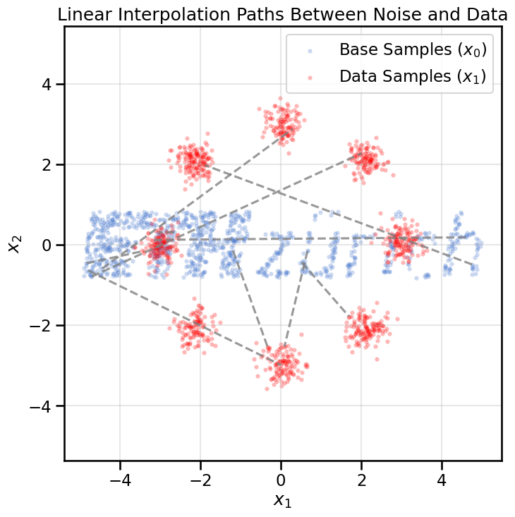
To understand what this synthetic coupling means, let’s visualize these straight-line paths.
Show Code
# Load datadata, labels = create_ring_gaussians(n_samples=1000)BASE_DISTRIBUTION ='ethz_logo'# Options: 'gaussian', 'uniform', 'ethz_logo'# Sample from base distributionif BASE_DISTRIBUTION =='gaussian': x0_samples = torch.randn(data.shape[0], 2)elif BASE_DISTRIBUTION =='uniform': x0_samples = torch.rand(data.shape[0], 2)*7.0-3.5# Uniform noise in [-3.5, 3.5]elif BASE_DISTRIBUTION =='ethz_logo': x0_samples = load_eth_z_logo_data(n_samples=data.shape[0])# Take a small subset to visualizen_viz =10x0_viz = x0_samples[:n_viz]x1_viz = torch.from_numpy(data[:n_viz]).float()plt.figure(figsize=(8, 8))plt.scatter(x0_samples[:, 0], x0_samples[:, 1], s=10, alpha=0.2, label='Base Samples ($x_0$)')plt.scatter(data[:, 0], data[:, 1], s=10, alpha=0.2, color='red', label='Data Samples ($x_1$)')# Draw lines connecting pairsfor i inrange(n_viz): plt.plot([x0_viz[i, 0], x1_viz[i, 0]], [x0_viz[i, 1], x1_viz[i, 1]], color='gray', linestyle='--', alpha=0.8)plt.title('Linear Interpolation Paths Between Noise and Data')plt.xlabel('$x_1$')plt.ylabel('$x_2$')plt.axis('equal')plt.legend()plt.grid(True, alpha=0.3)plt.show()
Each dashed line represents a simple path from a noise sample to a data sample. Our goal is to train a vector field that will push particles along these kinds of paths.
NoteWhy pick the pairs of points randomly?
It may first seem odd to randomly pair points from the base and data distributions. Why not try to find the ‘best’ matching pairs, as we did earlier when we covered Optimal Transport? In that chapter, we saw that by computing the optimal transport map, we could minimize the total cost of moving probability mass, which also seems like it would be useful in flow matching and lead to better paths. One major downside of Optimal Transport is that finding the optimal matching can be computationally expensive, especially in high dimensions or with large datasets. Flow Matching sidesteps this complexity by using completely random pairings as we can see above.
But why should this work? Does a velocity field trained on random pairings still learn to transport mass correctly from the base to the data distribution?
This was the main insight from the original Flow Matching paper by Lipman et al. (2022). They showed (see Appendix A) that even with random pairings, the expected velocity field learned over many such random pairs still approximates the true optimal transport interpolant needed to move mass from the base to the data distribution. Intuitively, while any single random pairing may not represent an optimal path, averaging over many such paths provides a good approximation of the overall flow needed to transform one distribution into the other. Of course, you could also use more sophisticated pairing strategies, such as actually computing the optimal transport coupling, but what was impressive about the original Flow Matching paper was that the random pairing approach is simple, efficient, and works surprisingly well in practice.
19.4 Training via Velocity Regression
The training objective for Flow Matching is a straightforward regression problem. We want our neural network \(v_\theta(x_t, t)\) to predict the true velocity, \(x_1 - x_0\), and the loss function is a simple Mean Squared Error:
This is even simpler than the diffusion model objective. There are no noise schedules (\(\alpha_t\), \(\beta_t\)) to worry about.
19.4.1 The Training Pipeline
The training process for each step is as follows:
Sample a Pair: Pick a noise sample \(x_0\) at random from the base distribution and a data sample \(x_1\) at random from the training data.
Sample Time: Pick a random timestep \(t\) uniformly from \([0, 1]\).
Interpolate: Compute the point on the path: \(x_t = (1-t)x_0 + t x_1\).
Compute Target Velocity: The target is simply \(v_{target} = x_1 - x_0\).
Predict Velocity: Feed \(x_t\) and \(t\) into the neural network \(v_\theta(x_t, t)\) to get the predicted velocity.
Compute Loss: Calculate the Mean Squared Error between the network’s prediction and the target velocity.
Update: Backpropagate and update the network’s weights.
Let’s implement this. The network architecture will be very similar to the one we used for our diffusion model, as it also needs to be conditioned on time.
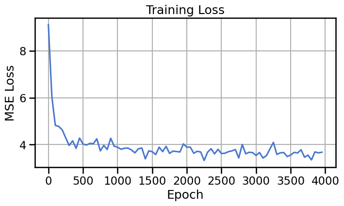
# Time-conditional network to predict velocityclass VelocityField(nn.Module):def__init__(self, time_emb_dim=16, hidden_dim=128):super().__init__()# We can't use an embedding layer for continuous time, so we'll use a small MLPself.time_mlp = nn.Sequential( nn.Linear(1, time_emb_dim), nn.ReLU(), nn.Linear(time_emb_dim, time_emb_dim), nn.ReLU(), nn.Linear(time_emb_dim, time_emb_dim) )self.net = nn.Sequential( nn.Linear(2+ time_emb_dim, hidden_dim), nn.ReLU(), nn.Linear(hidden_dim, hidden_dim), nn.ReLU(), nn.Linear(hidden_dim, hidden_dim), nn.ReLU(), nn.Linear(hidden_dim, hidden_dim), nn.ReLU(), nn.Linear(hidden_dim, 2) # Predicts the velocity vector )def forward(self, x, t):# t is expected to be of shape [batch_size, 1] t_emb =self.time_mlp(t) x_in = torch.cat([x, t_emb], dim=-1)returnself.net(x_in)# Training parameterslr =1e-3if BASE_DISTRIBUTION =='ethz_logo': n_epochs =4000else: n_epochs =500batch_size =1000loader = make_loader(data, batch_size=batch_size)# Model and optimizerflow_model = VelocityField().to(device)optimizer = optim.AdamW(flow_model.parameters(), lr=lr)# Training looplosses = []for epoch inrange(n_epochs):for (x1_batch,) in loader: x1 = x1_batch.to(device)# 1. Sample noiseif BASE_DISTRIBUTION =='gaussian': x0 = torch.randn_like(x1)elif BASE_DISTRIBUTION =='uniform': x0 = torch.rand_like(x1)*7.0-3.5# Uniform noise in [-3.5, 3.5]elif BASE_DISTRIBUTION =='ethz_logo': x0 = torch.Tensor(load_eth_z_logo_data(n_samples=x1.shape[0])) x0 = x0.to(device)# 2. Sample time t = torch.rand(x1.shape[0], 1, device=device)# 3. Interpolate xt = (1- t) * x0 + t * x1# 4. Compute target velocity target_v = x1 - x0# 5. Predict velocity predicted_v = flow_model(xt, t)# 6. Compute loss loss = nn.functional.mse_loss(predicted_v, target_v) optimizer.zero_grad() loss.backward() optimizer.step()if epoch %50==0: losses.append(loss.item())print(f"Epoch {epoch}, Loss: {loss.item():.4f}")print("Training complete.")# Plot the loss curveplt.figure(figsize=(8, 4))plt.plot(range(0, n_epochs, 50), losses)plt.title("Training Loss")plt.xlabel("Epoch")plt.ylabel("MSE Loss")plt.grid(True)plt.show()
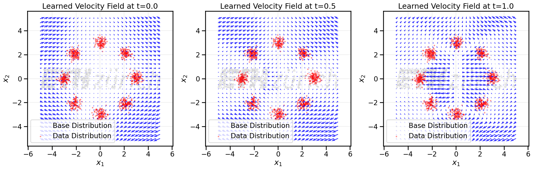
# Visualize the learned velocity fieldxx, yy = np.meshgrid(np.linspace(-5, 5, 30), np.linspace(-5, 5, 30))grid_points = torch.tensor(np.stack([xx.ravel(), yy.ravel()], axis=1), dtype=torch.float32, device=device)# Get the velocity at each grid point at different timesfig, axes = plt.subplots(1, 3, figsize=(18, 6))times_to_viz = [0.0, 0.5, 1.0]for idx, t_val inenumerate(times_to_viz): ax = axes[idx]# Create time tensor t_grid = torch.full((grid_points.shape[0], 1), t_val, device=device)# Get velocity predictions flow_model.eval()with torch.no_grad(): velocities = flow_model(grid_points, t_grid).cpu().numpy()# Plot base distribution samples in light greyif BASE_DISTRIBUTION =='gaussian': base_samples = np.random.randn(1000, 2)elif BASE_DISTRIBUTION =='uniform': base_samples = np.random.rand(1000, 2)*7.0-3.5# Uniform noise in [-3.5, 3.5]elif BASE_DISTRIBUTION =='ethz_logo': base_samples = load_eth_z_logo_data(n_samples=1000) ax.scatter(base_samples[:, 0], base_samples[:, 1], s=5, color='lightgrey', alpha=0.3, label='Base Distribution')# Plot data samples in red ax.scatter(data[:, 0], data[:, 1], s=5, color='red', alpha=0.3, label='Data Distribution')# Plot velocity field ax.quiver(grid_points[:, 0].cpu(), grid_points[:, 1].cpu(), velocities[:, 0], velocities[:, 1], color='blue', width=0.005, alpha=0.8) ax.set_title(f'Learned Velocity Field at t={t_val:.1f}') ax.set_xlabel('$x_1$') ax.set_ylabel('$x_2$') ax.axis('equal') ax.set_xlim(-5, 5) ax.set_ylim(-5, 5) ax.grid(True, alpha=0.2) ax.legend()plt.tight_layout()plt.show()
Ignoring fixed y limits to fulfill fixed data aspect with adjustable data limits.
Ignoring fixed y limits to fulfill fixed data aspect with adjustable data limits.
Ignoring fixed y limits to fulfill fixed data aspect with adjustable data limits.
Ignoring fixed x limits to fulfill fixed data aspect with adjustable data limits.
Ignoring fixed x limits to fulfill fixed data aspect with adjustable data limits.
Ignoring fixed x limits to fulfill fixed data aspect with adjustable data limits.
Show Code
def animate_velocity_field(model, grid_points, data, times=None, skip=1):"""Create an inline animation of the learned velocity field over time. model: a time-conditional velocity model taking (x, t) -> v grid_points: torch tensor of shape [N, 2] with points where to evaluate the field data: numpy array of data samples for background plotting times: 1D array-like of time values in [0,1]. If None, uses 101 steps. skip: sample every `skip` frames for the animation to speed it up. """if times isNone: times = np.linspace(0.0, 1.0, 101) times = np.asarray(times) model.eval() xx = grid_points[:, 0].cpu().numpy() yy = grid_points[:, 1].cpu().numpy() fig, ax = plt.subplots(figsize=(6, 6))def update(i): ax.clear() t_val =float(times[i]) t_grid = torch.full((grid_points.shape[0], 1), t_val, device=device)with torch.no_grad(): v = model(grid_points, t_grid).cpu().numpy()# Background: data samples in red ax.scatter(data[:, 0], data[:, 1], s=5, color='red', alpha=0.3)# Quiver plot of velocity field ax.quiver(xx, yy, v[:, 0], v[:, 1], color='blue', width=0.005, alpha=0.9) ax.set_title(f'Learned Velocity Field — t={t_val:.3f}') ax.set_xlim(-5, 5) ax.set_ylim(-5, 5) ax.set_xlabel('$x_1$') ax.set_ylabel('$x_2$') ax.set_aspect('equal', adjustable='box') ax.grid(True, alpha=0.2) frames =range(0, len(times), max(1, skip)) ani = FuncAnimation(fig, update, frames=frames, repeat=False, interval=80) plt.close(fig)return HTML(ani.to_jshtml())# Default call: show a 101-frame animation (sample every 2 frames to speed up)animate_velocity_field(flow_model, grid_points, data, times=np.linspace(0, 1, 101), skip=2)
19.5 Generating Samples by Solving the ODE
Once the velocity field \(v_\theta(x, t)\) is trained, we can generate samples by solving the initial value problem defined by our ODE. We start with a random sample from the base distribution, \(x_0 \sim \mathcal{N}(0, I)\), and integrate the velocity field from \(t=0\) to \(t=1\):
\[
x_1 = x_0 + \int_0^1 v_\theta(x_t, t) dt
\]
In practice, we use a numerical ODE solver to approximate this integral. A simple choice is the Euler method, where we take small, discrete steps in time:
We repeat this process from \(t=0\) to \(t=1\) to get our final sample. More sophisticated solvers like Runge-Kutta (RK4) can provide more accurate solutions with fewer steps.
Let’s implement a simple Euler integrator and use it to generate samples. We will animate the process to see the smooth, deterministic flow from noise to data.
@torch.no_grad()def generate_with_ode_solver(model, n_samples=500, n_steps=100, initial_noise_scale=1.0):"""Generate samples by solving the ODE with Euler's method. Note here that unlike in CNFs, we don't require the ODE solver to be differentiable, because we are only using it for sampling points not training. """ model.eval()# Start with pure noiseif BASE_DISTRIBUTION =='gaussian': x = torch.randn(n_samples, 2, device=device) * initial_noise_scaleelif BASE_DISTRIBUTION =='uniform': x = torch.rand(n_samples, 2, device=device)*7.0-3.5elif BASE_DISTRIBUTION =='ethz_logo': x = torch.tensor(load_eth_z_logo_data(n_samples=n_samples), dtype=torch.float32, device=device)# Store trajectory for animation trajectory = [x.cpu().numpy()] dt =1./ n_stepsfor i inrange(n_steps): t = torch.full((n_samples, 1), i / n_steps, device=device)# Predict velocity v = model(x, t)# Euler step x = x + v * dt trajectory.append(x.cpu().numpy())return x.cpu().numpy(), np.array(trajectory)# Generate samples and their trajectoriesgenerated_samples_flow, trajectory_flow = generate_with_ode_solver(flow_model, n_samples=1000, n_steps=500)
Show Code
# Create the animationfig, ax = plt.subplots(figsize=(8, 8))def update_flow(frame): ax.clear()# Plot the target distribution in the background#sns.kdeplot(x=data[:, 0], y=data[:, 1], cmap="viridis", fill=True, alpha=0.3, ax=ax, levels=15) ax.scatter(data[:, 0], data[:, 1], s=5, color='lightgrey', alpha=0.5)# Plot the current state of the samples current_samples = trajectory_flow[frame] ax.scatter(current_samples[:, 0], current_samples[:, 1], s=10, color='red', alpha=0.8) ax.set_title(f"Flow Matching: Step {frame}/{trajectory_flow.shape[0]-1}") ax.set_xlabel('$x_1$') ax.set_ylabel('$x_2$')#ax.axis('equal') ax.set_xlim(-5, 5) ax.set_ylim(-5, 5) ax.grid(True, alpha=0.2)# Create and display the animationskip_frames =10frames =range(0, trajectory_flow.shape[0], skip_frames)ani_flow = FuncAnimation(fig, update_flow, frames=frames, repeat=False, interval=50)plt.close(fig) # Prevent static plot from showingHTML(ani_flow.to_jshtml())
The animation shows the smooth, deterministic paths the samples take as they are pushed by the learned velocity field. Unlike the stochastic, zig-zagging paths of the diffusion sampler, these particles flow directly and efficiently toward the target distribution.
19.6 Conditional Generation with Flow Matching
As with diffusion models, Flow Matching can be extended to conditional generation tasks. By conditioning the velocity field on additional information (like class labels or text embeddings), we can guide the flow to generate samples that match specific conditions. For example, if we want to generate images of specific classes, we can modify our velocity network to take an additional input representing the class label. During training, we would sample pairs of points \((x_0, x_1)\) along with their corresponding class labels and train the network to predict the velocity conditioned on these labels. Likewise, during sampling, we would start with a noise sample and integrate the ODE while providing the desired condition to the velocity network at each step.
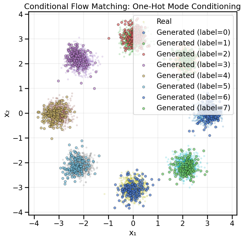
Below, we will repeat our earlier exercises on conditional generation, this time using Flow Matching instead of Diffusion Models. As before, we will first train on a discrete set of classes (the ring of Gaussians) and note how the learned flow fields change as we modify the conditioning label. Then we will show a continuous conditioning example, where we condition on a continuous variable (the radius) to show how flow matching can condition on continuous variables.
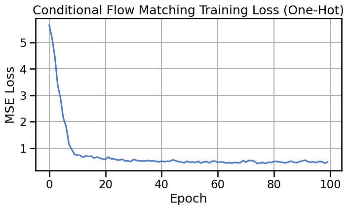
class ConditionalVelocityField(nn.Module):"""Velocity field conditioned on one-hot encoded mode labels."""def__init__(self, n_classes=8, time_emb_dim=16, hidden_dim=128):super().__init__()self.time_mlp = nn.Sequential( nn.Linear(1, time_emb_dim), nn.ReLU(), nn.Linear(time_emb_dim, time_emb_dim), nn.ReLU(), nn.Linear(time_emb_dim, time_emb_dim), )# Concatenate: x (2) + time_emb (time_emb_dim) + one_hot (n_classes)self.net = nn.Sequential( nn.Linear(2+ time_emb_dim + n_classes, hidden_dim), nn.ReLU(), nn.Linear(hidden_dim, hidden_dim), nn.ReLU(), nn.Linear(hidden_dim, hidden_dim), nn.ReLU(), nn.Linear(hidden_dim, hidden_dim), nn.ReLU(), nn.Linear(hidden_dim, 2), )def forward(self, x, t, c):""" Args: x: [batch, 2] - spatial coordinates t: [batch, 1] - time c: [batch, n_classes] - one-hot encoded class labels """ t_emb =self.time_mlp(t) x_in = torch.cat([x, t_emb, c], dim=-1)returnself.net(x_in)def train_conditional_flow_onehot( data, labels, n_epochs=500, batch_size=128, lr=1e-3, n_classes=8):"""Train the conditional velocity field with one-hot conditioning. """# Create conditional data loader cond_loader = make_conditional_loader_onehot( data=data, labels=labels, batch_size=batch_size, n_classes=n_classes )# Model and optimizer model = ConditionalVelocityField(n_classes=8).to(device) optimizer = optim.AdamW(model.parameters(), lr=lr)# Training loop losses = []for epoch inrange(n_epochs): epoch_loss =0.0 n_batches =0for x1_batch, labels_batch in cond_loader: x1 = x1_batch.to(device) c = labels_batch.to(device)# Sample noise x0 = torch.randn_like(x1)# Sample time t = torch.rand(x1.shape[0], 1, device=device)# Interpolate xt = (1- t) * x0 + t * x1# Compute target velocity target_v = x1 - x0# Predict velocity with conditioning predicted_v = model(xt, t, c)# Compute loss loss = nn.functional.mse_loss(predicted_v, target_v) optimizer.zero_grad() loss.backward() optimizer.step() epoch_loss += loss.item() n_batches +=1 avg_loss = epoch_loss / n_batches losses.append(avg_loss)if epoch %50==0:print(f"Epoch {epoch}, Loss: {avg_loss:.4f}")print("Conditional training complete.")# Plot the loss curve plt.figure(figsize=(8, 4)) plt.plot(range(n_epochs), losses) plt.title("Conditional Flow Matching Training Loss (One-Hot)") plt.xlabel("Epoch") plt.ylabel("MSE Loss") plt.grid(True) plt.show()return model@torch.no_grad()def sample_conditional_flow(model, condition, n_samples=100, n_steps=100):"""Generate samples using conditional flow matching. Args: model: Conditional velocity field model condition: [batch, n_classes] one-hot encoded condition n_samples: Number of samples to generate n_steps: Number of ODE integration steps """ model.eval()# Start with pure noise x = torch.randn(n_samples, 2, device=device)# Expand condition to match batch size c = condition.repeat(n_samples, 1) dt =1.0/ n_stepsfor i inrange(n_steps): t = torch.full((n_samples, 1), i / n_steps, device=device) v = model(x, t, c) x = x + v * dtreturn x.cpu().numpy()def visualize_conditional_samples_onehot(model, n_modes=8, n_samples_per_mode=200):"""Generate and visualize samples for each mode."""# Build samples dict expected by the utility plotting function samples_by_label = {}for mode_idx inrange(n_modes): condition = torch.zeros(1, n_modes, device=device) condition[0, mode_idx] =1.0 samples = sample_conditional_flow( model, condition, n_samples=n_samples_per_mode ) samples_by_label[int(mode_idx)] = samples# Load reference real data for background and labels real_data, real_labels = create_ring_gaussians(n_samples=5000, n_modes=n_modes)# Visualize using utilities (expects dict and real data/labels) plot_conditional_samples_discrete( samples_by_label, real_data=real_data, real_labels=real_labels, title="Conditional Flow Matching: One-Hot Mode Conditioning", )
# Train conditional model with one-hot encodingmodel_onehot = train_conditional_flow_onehot(data = data, labels=labels, n_epochs=100, batch_size=128, lr=1e-3)# Visualize resultsvisualize_conditional_samples_onehot( model_onehot, n_modes=8, n_samples_per_mode=200)
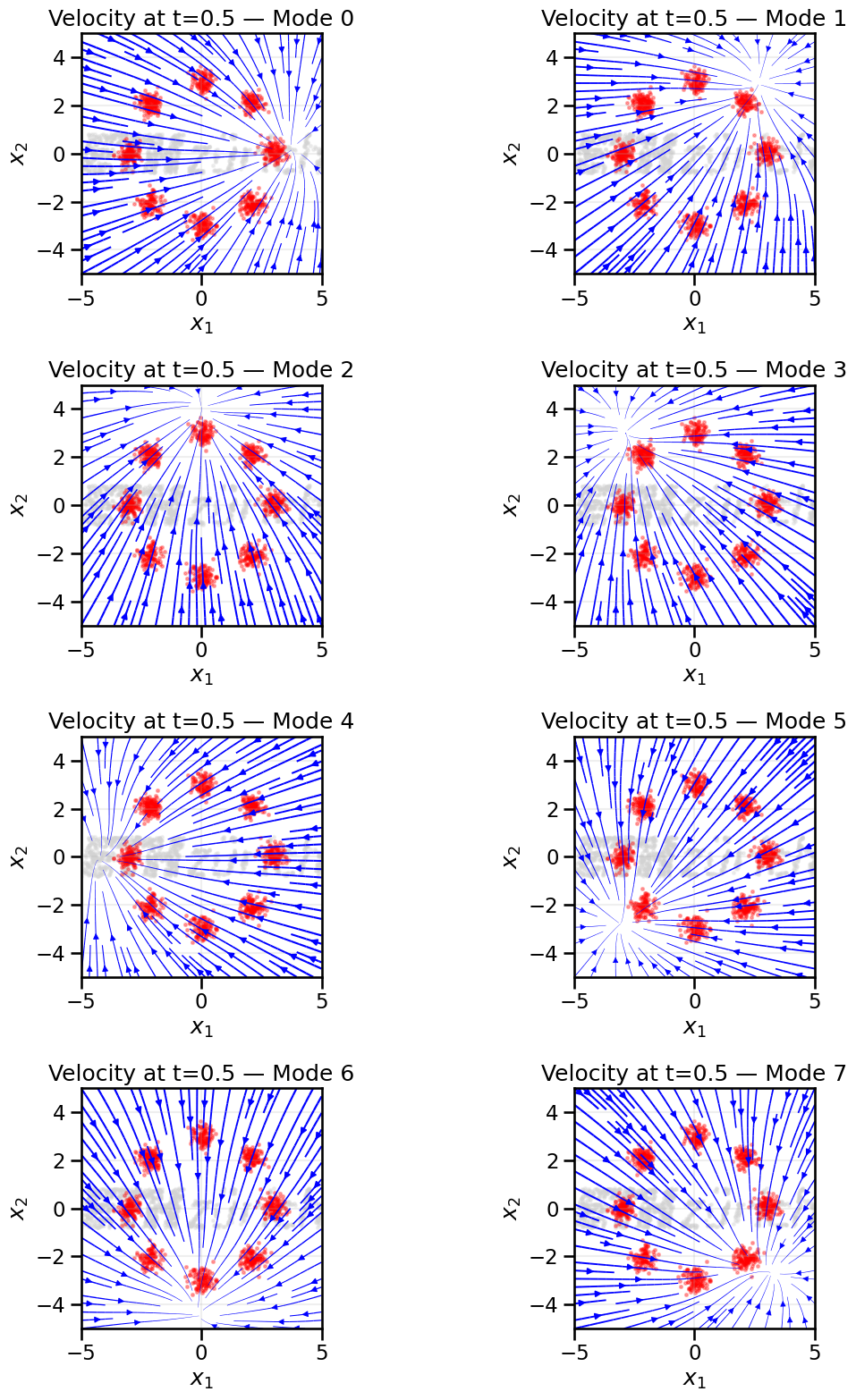
By looking at the flow fields below, we can see how the conditioning label influences the direction and magnitude of the velocity vectors, guiding samples toward the desired mode in the ring of Gaussians example.
Show Code
# Check the corresponding learned vector fields for each conditionn_classes =8xx, yy = np.meshgrid(np.linspace(-5, 5, 20), np.linspace(-5, 5, 20))grid_points = torch.tensor(np.stack([xx.ravel(), yy.ravel()], axis=1), dtype=torch.float32, device=device)# Create a 2-column, 4-row figure and plot each mode into a subplotfig, axes = plt.subplots(4, 2, figsize=(12, 16))axes = axes.ravel()# Prepare base samples once (same as before)if BASE_DISTRIBUTION =='gaussian': base_samples = np.random.randn(1000, 2)elif BASE_DISTRIBUTION =='uniform': base_samples = np.random.rand(1000, 2) *7.0-3.5elif BASE_DISTRIBUTION =='ethz_logo': base_samples = load_eth_z_logo_data(n_samples=1000)for mode_idx inrange(n_classes): ax = axes[mode_idx] condition = torch.zeros(1, n_classes, device=device) condition[0, mode_idx] =1.0 c_grid = condition.repeat(grid_points.shape[0], 1)# Get the velocity at each grid point at time t=0.5 t_grid = torch.full((grid_points.shape[0], 1), 0.5, device=device) flow_model.eval()with torch.no_grad(): velocities = model_onehot(grid_points, t_grid, c_grid).cpu().numpy()# Background: base and data ax.scatter(base_samples[:, 0], base_samples[:, 1], s=5, color='lightgrey', alpha=0.3, label='Base Distribution') ax.scatter(data[:, 0], data[:, 1], s=5, color='red', alpha=0.3, label='Data Distribution')# Quiver replaced by streamlines for smoother visualization# Reshape predicted velocities back to the grid shape expected by streamplot U = velocities[:, 0].reshape(xx.shape) V = velocities[:, 1].reshape(xx.shape)# Compute speed for linewidth scaling (avoid div-by-zero) speed = np.sqrt(U**2+ V**2) max_speed = speed.max() if speed.max() >0else1.0 linewidths =1.5* (speed / max_speed +0.1) # add small offset so thin vectors are visible# Plot streamlines strm = ax.streamplot( xx, yy, U, V, color='blue', linewidth=linewidths, density=1.0, arrowsize=1.0, arrowstyle='-|>', maxlength=6.0 ) ax.set_title(f'Velocity at t=0.5 — Mode {mode_idx}') ax.set_xlabel('$x_1$') ax.set_ylabel('$x_2$') ax.set_xlim(-5, 5) ax.set_ylim(-5, 5) ax.set_aspect('equal', adjustable='box') ax.grid(True, alpha=0.2)#ax.legend(loc='upper right')# If there are any unused subplots (shouldn't be here for 8 modes) hide themfor i inrange(n_classes, len(axes)): axes[i].axis('off')plt.tight_layout()plt.show()
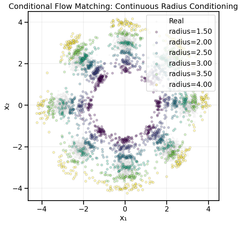
19.6.1 Example 2: Conditioning on the Continuous Radius
class ConditionalVelocityFieldRadius(nn.Module):"""Velocity field conditioned on continuous radius values."""def__init__(self, time_emb_dim=16, radius_emb_dim=16, hidden_dim=128):super().__init__()self.time_mlp = nn.Sequential( nn.Linear(1, time_emb_dim), nn.ReLU(), nn.Linear(time_emb_dim, time_emb_dim), nn.ReLU(), nn.Linear(time_emb_dim, time_emb_dim), )self.radius_mlp = nn.Sequential( nn.Linear(1, radius_emb_dim), nn.ReLU(), nn.Linear(radius_emb_dim, radius_emb_dim), nn.ReLU(), nn.Linear(radius_emb_dim, radius_emb_dim), )# Concatenate: x (2) + time_emb + radius_embself.net = nn.Sequential( nn.Linear(2+ time_emb_dim + radius_emb_dim, hidden_dim), nn.ReLU(), nn.Linear(hidden_dim, hidden_dim), nn.ReLU(), nn.Linear(hidden_dim, hidden_dim), nn.ReLU(), nn.Linear(hidden_dim, hidden_dim), nn.ReLU(), nn.Linear(hidden_dim, 2), )def forward(self, x, t, r):""" Args: x: [batch, 2] - spatial coordinates t: [batch, 1] - time r: [batch, 1] - radius values """ t_emb =self.time_mlp(t) r_emb =self.radius_mlp(r) x_in = torch.cat([x, t_emb, r_emb], dim=-1)returnself.net(x_in)def train_conditional_flow_radius(data, n_epochs=500, batch_size=128, lr=1e-3):"""Train the conditional velocity field with radius conditioning. """# if data is None:# data, _ = create_ring_gaussians(n_samples=5000)# Create conditional data loader with radius radius_loader = make_conditional_loader_radius(data=data, batch_size=batch_size)# Model and optimizer model = ConditionalVelocityFieldRadius().to(device) optimizer = optim.AdamW(model.parameters(), lr=lr)# Training loop losses = []for epoch inrange(n_epochs): epoch_loss =0.0 n_batches =0for x1_batch, radius_batch in radius_loader: x1 = x1_batch.to(device) r = radius_batch.to(device)# Sample noise x0 = torch.randn_like(x1)# Sample time t = torch.rand(x1.shape[0], 1, device=device)# Interpolate xt = (1- t) * x0 + t * x1# Compute target velocity target_v = x1 - x0# Predict velocity with radius conditioning predicted_v = model(xt, t, r)# Compute loss loss = nn.functional.mse_loss(predicted_v, target_v) optimizer.zero_grad() loss.backward() optimizer.step() epoch_loss += loss.item() n_batches +=1 avg_loss = epoch_loss / n_batches losses.append(avg_loss)if epoch %50==0:print(f"Epoch {epoch}, Loss: {avg_loss:.4f}")print("Conditional training with radius complete.")# Plot the loss curve plt.figure(figsize=(8, 4)) plt.plot(range(n_epochs), losses) plt.title("Conditional Flow Matching Training Loss (Radius)") plt.xlabel("Epoch") plt.ylabel("MSE Loss") plt.grid(True) plt.show()return model@torch.no_grad()def sample_conditional_flow_radius(model, radius_value, n_samples=100, n_steps=100):"""Generate samples using conditional flow matching with radius conditioning. Args: model: Conditional velocity field model radius_value: Scalar radius value to condition on n_samples: Number of samples to generate n_steps: Number of ODE integration steps """ model.eval()# Start with pure noise x = torch.randn(n_samples, 2, device=device)# Create radius condition r = torch.full((n_samples, 1), radius_value, device=device) dt =1.0/ n_stepsfor i inrange(n_steps): t = torch.full((n_samples, 1), i / n_steps, device=device) v = model(x, t, r) x = x + v * dtreturn x.cpu().numpy()def visualize_conditional_samples_radius( model, radius_values=None, n_samples_per_radius=200):"""Generate and visualize samples at different radius values."""if radius_values isNone: radius_values = [1.0, 1.5, 2.0, 2.5, 3.0, 3.5] samples_by_value = {}for radius_val in radius_values: samples = sample_conditional_flow_radius( model, radius_val, n_samples=n_samples_per_radius ) samples_by_value[float(radius_val)] = samples# Load real data for background real_data, _ = create_ring_gaussians(n_samples=5000)# Visualize plot_conditional_samples_continuous( samples_by_value, real_data=real_data, title="Conditional Flow Matching: Continuous Radius Conditioning", )
Show Code
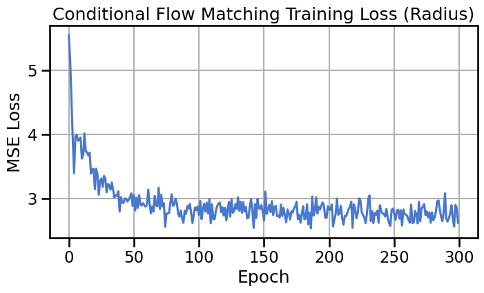
# Train conditional model with radiusmodel_radius = train_conditional_flow_radius(data=data,n_epochs=300, batch_size=128, lr=1e-3)
Flow Matching combines some of the best aspects of both Normalizing Flows and Diffusion Models:
Aspect
Diffusion Models
Normalizing Flows (CNF)
Flow Matching
Dynamics
Stochastic (SDE)
Deterministic (ODE)
Deterministic (ODE)
Training
Score/Noise Regression
Max Likelihood (trace)
Velocity Regression
Path
Random, noisy
Invertible, complex
Simple, straight-line
Sampling Speed
Slow (many steps)
Fast (single pass)
Fast (few ODE steps)
Stability
Very stable
Can be unstable
Very stable
Flow Matching avoids the expensive trace computation of CNFs and the slow, stochastic sampling of diffusion models. It provides a stable, efficient, and conceptually simple way to learn a generative model.
Flow Matching vs. Diffusion: Flow Matching learns a deterministic ODE, while diffusion models learn to reverse a stochastic SDE. This leads to faster, noise-free sampling.
Simple Training: The model is trained by regressing a time-conditional neural network on the simple velocity vector defined by a straight-line path between noise and data samples.
ODE-based Generation: Samples are generated by integrating the learned velocity field from \(t=0\) to \(t=1\) using a numerical ODE solver.
Through this part of the book we have covered a wide variety of generative models, ranging from GANs to VAEs, Normalizing Flows, Diffusion Models, and now Flow Matching. Yet many of these models struggle in high-dimensional settings. A popular and commonly used approach is to combine these Generative Models with reduced or latent dimensional representations, such as those learned by Autoencoders or Variational Autoencoders. In the next chapter we will see how to combine these two threads together to produce “Latent Generative Models”, such as Latent Diffusion Models or Latent Flow Models, which leverage the strengths of both generative modeling and representation learning.