12  Problem Set 1

12.1 PS1 Part 1: Linear Models and Validation

12.1.1 Preamble

We’ll be loading some CO2 concentration data that is a commonly used dataset for model building of time series prediction. You will build a few baseline linear models and assess them using some of the tools we discussed in class. Which model is best? Let’s find out.

First let’s just load the data and take a look at it:

import numpy as np
from matplotlib import pyplot as plt
import seaborn as sns
from sklearn.datasets import fetch_openml
from datetime import datetime, timedelta
import pandas as pd
from pandas.plotting import register_matplotlib_converters
register_matplotlib_converters()
sns.set_context('notebook')

# Fetch the data
mauna_lao = fetch_openml('mauna-loa-atmospheric-co2', as_frame = False)
print(mauna_lao.DESCR)
data = mauna_lao.data
# Assemble the day/time from the data columns so we can plot it
d1958 = datetime(year=1958,month=1,day=1)
time = [datetime(int(d[0]),int(d[1]),int(d[2])) for d in data]
X = np.array([1958+(t-d1958)/timedelta(days=365.2425) for t in time]).T
X = X.reshape(-1,1)  # Make it a column to make scikit happy
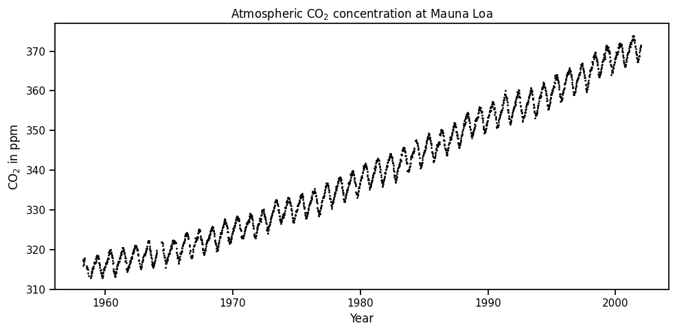
y = np.array(mauna_lao.target)

**Weekly carbon-dioxide concentration averages derived from continuous air samples for the Mauna Loa Observatory, Hawaii, U.S.A.**<br><br>
These weekly averages are ultimately based on measurements of 4 air samples per hour taken atop intake lines on several towers during steady periods of CO2 concentration of not less than 6 hours per day; if no such periods are available on a given day, then no data are used for that day. The _Weight_ column gives the number of days used in each weekly average. _Flag_ codes are explained in the NDP writeup, available electronically from the [home page](http://cdiac.ess-dive.lbl.gov/ftp/trends/co2/sio-keel-flask/maunaloa_c.dat) of this data set. CO2 concentrations are in terms of the 1999 calibration scale (Keeling et al., 2002) available electronically from the references in the NDP writeup which can be accessed from the home page of this data set.
<br><br>
### Feature Descriptions
_co2_: average co2 concentration in ppvm <br>
_year_: year of concentration measurement <br>
_month_: month of concentration measurement <br>
_day_: day of month of concentration measurement <br>
_weight_: number of days used in each weekly average <br>
_flag_: flag code <br>
_station_: station code <br>
<br>
**Author**: Carbon Dioxide Research Group, Scripps Institution of Oceanography, University of California-San Diego, La Jolla, California, USA 92023-0444 <br>
**Source**: [original](http://cdiac.ess-dive.lbl.gov/ftp/trends/co2/sio-keel-flask/maunaloa_c.dat) - September 2004

Downloaded from openml.org.

# Plot the data
plt.figure(figsize=(10,5))    # Initialize empty figure
plt.scatter(X, y, c='k',s=1) # Scatterplot of data
plt.xlabel("Year")
plt.ylabel(r"CO$_2$ in ppm")
plt.title(r"Atmospheric CO$_2$ concentration at Mauna Loa")
plt.tight_layout()
plt.show()

y[:100]

array([316.1, 317.3, 317.6, 317.5, 316.4, 316.9, 317.5, 317.9, 315.8,
       315.8, 315.4, 315.5, 315.6, 315.1, 315. , 314.1, 313.5, 313. ,
       313.2, 313.5, 314. , 314.5, 314.4, 314.7, 315.2, 315.2, 315.5,
       315.6, 315.8, 315.4, 316.9, 316.6, 316.6, 316.8, 316.7, 316.7,
       317.7, 317.1, 317.6, 318.3, 318.2, 318.7, 318. , 318.4, 318.5,
       318.1, 317.8, 317.7, 316.8, 316.8, 316.4, 316.1, 315.6, 314.9,
       315. , 314.1, 314.4, 313.9, 313.5, 313.5, 313. , 313.1, 313.4,
       313.4, 314.1, 314.4, 314.8, 315.2, 315.1, 315. , 315.6, 315.8,
       315.7, 315.7, 316.4, 316.7, 316.5, 316.6, 316.6, 316.9, 317.4,
       317. , 316.9, 317.7, 318. , 317.7, 318.6, 319.3, 319. , 319. ,
       319.7, 319.9, 319.8, 320. , 320. , 319.4, 320. , 319.4, 319. ,
       318.1])

12.1.2 Linear Models

Construct the following linear models: 1. Model 1: “Vanilla” Linear Regression, that is, where \(CO_2 = a+b \cdot time\) 2. Model 2: Quadratic Regression, where \(CO_2 = a+b \cdot t + c\cdot t^2\) 3. Model 3: A more complex “linear” model with the following additive terms \(CO_2=a+b\cdot t+c\cdot sin(\omega\cdot t)\): * a linear (in time) term * a sinusoidal additive term with period such that the peak-to-peak of the sinsusoid is roughly ~1 year and phase shift of zero (set \(\omega\) as appropriate to match the peaks) 4. Model 4: A “linear” model with the following additive terms (\(CO_2=a+b\cdot t+c\cdot t^2+d\cdot sin(\omega\cdot t)\): * a quadratic (in time) polynomial * a sinusoidal additive term with period such that the peak-to-peak of the sinsusoid is roughly ~1 year and phase shift of zero (set \(\omega\) as appropriate to match the peaks)

Evauate these models using the appropriate kind of Cross Validation for each of the following amounts of Training data: 1. N=50 Training Data Points 2. N=100 3. N=200 4. N=500 5. N=1000 6. N=2000

Question: Before you even construct the models or do any coding below, what is your initial guess or intuition behind how each of those four models will perform? Note: there is no right or wrong answer to this part of the assignment and this question will only be graded on completeness, not accuracy. It’s intent is to get you to think about and write down your preliminary intuition regarding what you think will happen before you actually implement anything, based on your approximate understanding of how functions of the above complexity should perform as N increases.

Student Response: [Insert your response here]

Question: What is the appropriate kind of Cross Validation to perform in this case if we want a correct Out of Sample estimate of our Test MSE?

Student Response: [Insert your response here]

Now, for each of the above models and training data sizes: * Plot the predicted CO2 as a function of time, including the actual data, for each of the N=X training data examples. This should correspond to six plots (one for each amount of training data) if you plot all models on the same plot, or 6x4 = 24 plots if you plot each model and training data plot separately. * Create a Learning Curve plot for the model which plots its Training and Test MSE as a function of training data. That is, plot how Training and Testing MSE change as you increase the training data for each model. This could be a single plot for all four models (8 lines on the plot) or four different plots corresponding to the learning curve of each model separately.

import numpy as np

X_train_100 = X[:100]
y_train_100 = y[:100]
X_test = X[100:200]
print("Shape of X_train_100: %s" % str(X_train_100.shape))
print("Beginning of X_train_100: %s" % str(X_train_100[0:5]))
print("Shape of y_train_100: %s" % str(y_train_100.shape))
print("Beginning of y_train_100: %s" % str(y_train_100[0:5]))

print('Shape of X_test: %s' % str(X_test.shape))
print("Beginning of X_test: %s" % str(X_test[0:5]))

### Modify the below code. You can leave the code above as is. ###

Shape of X_train_100: (100, 1)
Beginning of X_train_100: [[1958.23819791]
 [1958.25736326]
 [1958.27652861]
 [1958.29569396]
 [1958.31485931]]
Shape of y_train_100: (100,)
Beginning of y_train_100: [316.1 317.3 317.6 317.5 316.4]
Shape of X_test: (100, 1)
Beginning of X_test: [[1960.51887445]
 [1960.5380398 ]
 [1960.55720514]
 [1960.57637049]
 [1960.59553584]]

# Insert Modeling Building or Plotting code here
# Note, you may implement these however you see fit
# Ex: using an existing library, solving the Normal Eqns
#     implementing your own SGD solver for them. Your Choice.
from sklearn.linear_model import SGDRegressor, LinearRegression
sgd = SGDRegressor()
lr = LinearRegression()

sgd.fit(X,y)
lr.fit(X,y)

LinearRegression()

sgd.predict(X)

array([-1.78959753e+15, -1.78961505e+15, -1.78963256e+15, ...,
       -1.82954889e+15, -1.82956640e+15, -1.82958392e+15])

lr.predict(X)

array([310.2080183 , 310.23375578, 310.25949326, ..., 368.9152125 ,
       368.94094999, 368.96668747])

Question: Which Model appears to perform best in the N=50 or N=100 Condition? Why is this?

Student Response: [Insert your response here]

Question: Which Model appears to perform best as the N=200 to 500? Why is this?

Student Response: [Insert your response here]

Question: Which Model appears to perform best as N = 2000? Why is this?

Student Response: [Insert your response here]

12.2 PS1 Part 2: Unsupervised Linear Models

12.2.1 Toy Dataset

For this problem, you will use the data file hb.csv. The input is 2,280 data points, each of which is 7 dimensional (i.e., input csv is 2280 rows by 7 columns). Use Principal Component Analysis (either an existing library, or through your own implementation by taking the SVD of the Covariance Matrix) for the follow tasks.

%matplotlib inline
import pandas
url = "https://raw.githubusercontent.com/IDEALLab/ML4ME_Textbook/main/problems/hb.csv"
data = pandas.read_csv(url,header=None)
#data.head()

12.2.2 Task 1

Assuming that the 7-dimensional space is excessive, you would like to reduce the dimension of the space. However, what dimensionality of space should we reduce it to? To determine this we need to compute its intrinsic dimensionality. Plot the relative value of the information content of each of the principal components and compare them.

Note: this information content is called the “explained variance” of each component, but you can also get this from the magnitude of the singular values. This plot is sometimes called a “Scree Plot”.

# Code Here

Question: Approximately how many components dominate the space?, and what does this tell us about the intrinsic dimensionality of the space?

Response:

12.2.2.1 Task 2

Now use PCA to project the 7-dimensional points on the K-dimensional space (where K is your answer from above) and plot the points. (For K=1,2, or 3, use a 1, 2, or 3D plot, respectively. For 4+ dimensions, use a grid of pairwise 2D Plots, like the Scatter Matrix we used in class).

# Code Here

Question: What do you notice?

Response:

12.2.3 Topology Optimization Dataset

For this problem, you will be using unsupervised linear models to help understand and interpret the results of a mechanical optimization problem. Specifically, to understand the solution space generated by a topology optimization code; that is, the results of finding the optimal geometries for minimizing the compliance of various bridge structures with different loading conditions. The input consists of 1,000 images of optimized material distribution for a beam as described in Figure 1. A symmetrical boundary condition, left side, is used to reduce the analysis to only half. Also, a rolling support is included at the lower right corner. Notice that the rolling support is the only support in the vertical direction.

 

Figure 1: Left: Nx-by-Ny design domain for topology optimization problem. Right: Example loading configuration and resulting optimal topology. Two external forces, Fi, were applied to the beam at random nodes represented by (xi, yi) coordinates.¹

 

Use Principal Component Analysis (either an existing library, or through your own implementation by taking the SVD of the Covariance Matrix) for the follow tasks.

^{1. This problems data is based on the problem setup seen in the following paper: Ulu, E., Zhang, R., & Kara, L. B. (2016). A data-driven investigation and estimation of optimal topologies under variable loading configurations. Computer Methods in Biomechanics and Biomedical Engineering: Imaging & Visualization, 4(2), 61-72.}

# To help you get started, the below code will load the images from the associated image folder:
%matplotlib inline
import numpy as np
import matplotlib.pyplot as plt
import os
from PIL import Image
import requests, zipfile, io

#im_dir = './topo_opt_runs/'
url = "https://raw.githubusercontent.com/IDEALLab/ML4ME_Textbook/main/problems/topo_opt_runs.zip"
resp = requests.get(url)
resp.raise_for_status()
zf = zipfile.ZipFile(io.BytesIO(resp.content))

images = []
for name in sorted(zf.namelist()):
    with zf.open(name) as f:
        img = Image.open(f).convert('L')
        images.append(np.asarray(img))

height,width = images[0].shape
print('The images are {:d} pixels high and {:d} pixels wide'.format(height,width))

# Print matrix corresponding to the image:
print(images[-1])
# And show example image, so you can see how matrix correponds:
img

The images are 217 pixels high and 434 pixels wide
[[  0   0   0 ... 255 255 255]
 [  0   0   0 ... 255 255 255]
 [  0   0   0 ... 255 255 255]
 ...
 [  0   0   0 ...   0   0   0]
 [  0   0   0 ...   0   0   0]
 [  0   0   0 ...   0   0   0]]

12.2.4 Task 1: Scree/Singular Value Plot

As with the toy example, assume that the 94,178-dimensional space is excessive. You would like to reduce the dimension of the image space. First compute its intrinsic dimensionality. For this application, “good enough” means capturing 95% of the variance in the dataset. How many dimensions are needed to capture at least 95% of the variance in the provided dataset? Store your answer in numDimsNeeded. (Hint: A Scree plot may be helpful, though visual inspection of a graph may not be precise enough.)

Question: Approximately how many components dominate the space? What does this tell us about the intrinsic dimensionality of the space?

Response:

12.2.5 Task 2: Principal Components

Now plot the first 5 principal components. Hint: looking at each of these top 5 principal components; do they make sense physically, in terms of what it means for where material in the bridge is placed? Compare, for example, the differences between the 1st and 2nd principal component?

12.3 PS1 Part 3: Bi-Linear Models and SGD

12.3.1 Bilinear Models for Recommendation

For this problem, you will derive a very simple recommendation system that uses a combination of unsupervised and supervised approachs and demonstrates use of Stochastic Gradient Descent.

Specifically, in class we discussed recommender models of the form: \[ f(user,movie) = \langle v_u,v_m \rangle + b_u + b_m + \mu \]

where \(v\) is a vector that represents a user’s or movie’s location in an N-Dimensional space, \(b\) is a vector that represents a specific “bias” term fo r each movie and user, and \(\mu\) is a scalar that represents a kind of global anchor or base score (i.e., a sort of average movie rating). This means that each user has two vectors (e.g., \(v_{\mathrm{jack~smith}}\) and \(b_{\mathrm{jack~smith}}\)), and each movie has two vectors (e.g., \(v_{\mathrm{Avengers}}\) and \(b_{\mathrm{Avengers}}\)), with each of those vectors being N-Dimensional (in class we used two dimensions). For this, we constructed a loss function as follows: \[ Cost = Loss + Penalty \] where \[ Loss = \Sigma_{(u,m)\in \mathrm{Ratings}} \frac{1}{2}\left( \langle v_u,v_m \rangle + b_u + b_m + \mu - y_{u,m}\right)^2 \] and \[ Penalty = \frac{\lambda}{2}\left(\Sigma_u \left[\| v_u\|^2_2 + b_u^2\right] + \Sigma_m \left[\|v_m\|^2_2 + b_m^2\right]\right) \]

12.3.2 Task 1: Analytical Gradients

To use stochastic gradient descent, we first need to write down the gradients. Using the above cost function (including both the loss and penalty), compute the following partial derivatives:

\[ \frac{\partial \textrm{Cost}}{\partial v_u } = \]

\[ \frac{\partial \textrm{Cost}}{\partial v_m } = \]

\[ \frac{\partial \textrm{Cost}}{\partial b_u} = \]

\[ \frac{\partial \textrm{Cost}}{\partial b_m} = \]

\[ \frac{\partial \textrm{Cost}}{\partial \mu} = \]

You can either do this directly in the notebook using LaTeX notation, or via a scanned image. Please remember to show your work in how you computed the derivatives, not just the final result. Note: Recall that the partial derivative of e.g. Nicholas’s rating on Titanic with respect to the user Mark would be zero. When computing your SGD updates, consider how this might impact individual terms for users and movies in the loss function.

12.3.3 Task 2: Stochastic Gradient Descent

Now you are actually going to implement SGD on this type of model and optimize it until convergence on a toy dataset. To simplify the implementation, we’ll actually make the model a little simpler than the one you derived updates for in task 1. Specifically, we’ll just use:

\[ Cost = \Sigma_{(u,m)\in \mathrm{Ratings}} \frac{1}{2}\left( \langle v_u,v_m \rangle + \mu - y_{u,m}\right)^2 + \frac{\lambda}{2}\left(\| v_u\|^2_2 + \|v_m\|^2_2\right) \]

This way all you have to estimate is two vectors — \(v_u\) for each user and \(v_m\) for each movie — and \(\mu\) — a scalar value similar to an average rating. For simplicity, we’ll assume here that the size of the latent space (K) is 2 (i.e., the length of each \(v_u\) & \(v_m\)).

Using your above gradients, write down the update equations for each vector using stochastic gradient descent. Once you have done this, implement those update equations in code like we did in the in-class notebook. For simplicity, you can just use a constant step size \(\alpha\) if you wish, though you may change this if you want. Note: depending on exactly how you implement your model and what batch size you use, i.e., one point at a time, or some subset of data points, values of \(\alpha\) anywhere between around 0.7 and 0.01 should be sufficient to converge the model in under 1000 epochs, i.e., passes through the dataset. If you implement more advanced tricks covered in some optional readings this can converge much faster, but that is not necessary for this assignment, and it does not matter to me how quickly your model coverges, so long as it does so.

Use the below small sample dataset of movie ratings for five users and six movies to perform stochastic gradient descent to update those vectors until your model converges. To initialize your SGD, you can use the initial weights/terms we provide below, or you can initialize the model any other way you wish – the exact initialization should not make a big difference here.

# Your Code below!

import numpy as np
import pandas as pd
missing_ratings = pd.read_csv('missing.csv')
ratings = pd.read_csv('ratings.csv')
ratings

	movie	user	ratings
0	The Avengers	Alex	3.0
1	The Avengers	Priya	3.5
2	The Avengers	Yichen	3.5
3	When Harry Met Sally	Alex	3.0
4	When Harry Met Sally	Sally	4.5
5	When Harry Met Sally	Priya	3.0
6	When Harry Met Sally	Yichen	3.0
7	Silence of the Lambs	Alex	3.0
8	Silence of the Lambs	Sally	4.0
9	Silence of the Lambs	Juan	3.5
10	Silence of the Lambs	Priya	3.0
11	Silence of the Lambs	Yichen	2.5
12	Shawshank Redemption	Juan	2.5
13	Shawshank Redemption	Priya	4.0
14	Shawshank Redemption	Yichen	4.0
15	The Hangover	Alex	3.0
16	The Hangover	Sally	3.5
17	The Hangover	Priya	3.0
18	The Hangover	Yichen	2.5
19	The Godfather	Alex	3.0
20	The Godfather	Priya	3.5

# Alternatively, if you prefer, you can convert it into numpy first:
ratings_numpy = ratings.to_numpy()
ratings_numpy

array([['The Avengers', 'Alex', 3.0],
       ['The Avengers', 'Priya', 3.5],
       ['The Avengers', 'Yichen', 3.5],
       ['When Harry Met Sally', 'Alex', 3.0],
       ['When Harry Met Sally', 'Sally', 4.5],
       ['When Harry Met Sally', 'Priya', 3.0],
       ['When Harry Met Sally', 'Yichen', 3.0],
       ['Silence of the Lambs', 'Alex', 3.0],
       ['Silence of the Lambs', 'Sally', 4.0],
       ['Silence of the Lambs', 'Juan', 3.5],
       ['Silence of the Lambs', 'Priya', 3.0],
       ['Silence of the Lambs', 'Yichen', 2.5],
       ['Shawshank Redemption', 'Juan', 2.5],
       ['Shawshank Redemption', 'Priya', 4.0],
       ['Shawshank Redemption', 'Yichen', 4.0],
       ['The Hangover', 'Alex', 3.0],
       ['The Hangover', 'Sally', 3.5],
       ['The Hangover', 'Priya', 3.0],
       ['The Hangover', 'Yichen', 2.5],
       ['The Godfather', 'Alex', 3.0],
       ['The Godfather', 'Priya', 3.5]], dtype=object)

Let’s initialize the vectors to some random numbers, and \(\mu\) to 2.5

K=2
user_names = ratings['user'].unique()
movie_names = ratings['movie'].unique()
mu= 2.5
# Setting the seed of the random generator to a value so that everyone sees the same initialization
# should should be able to comment out the below with no ill-effects on whatever model you implement
# this may just help us in office hours if folks have difficulty implementing things
np.random.seed(0)
V = pd.DataFrame(np.random.random((len(user_names)+len(movie_names),K)),index=np.hstack([user_names,movie_names]))
print(V)

                             0         1
Alex                  0.548814  0.715189
Priya                 0.602763  0.544883
Yichen                0.423655  0.645894
Sally                 0.437587  0.891773
Juan                  0.963663  0.383442
The Avengers          0.791725  0.528895
When Harry Met Sally  0.568045  0.925597
Silence of the Lambs  0.071036  0.087129
Shawshank Redemption  0.020218  0.832620
The Hangover          0.778157  0.870012
The Godfather         0.978618  0.799159

# Here is one example of how to go through rows of a ratings matrix
for index, rating in ratings.iterrows():
    user  = rating['user']
    movie = rating['movie']
    score = rating['ratings']
    print(f"{user} gave {movie} a score of {score}")

Alex gave The Avengers a score of 3.0
Priya gave The Avengers a score of 3.5
Yichen gave The Avengers a score of 3.5
Alex gave When Harry Met Sally a score of 3.0
Sally gave When Harry Met Sally a score of 4.5
Priya gave When Harry Met Sally a score of 3.0
Yichen gave When Harry Met Sally a score of 3.0
Alex gave Silence of the Lambs a score of 3.0
Sally gave Silence of the Lambs a score of 4.0
Juan gave Silence of the Lambs a score of 3.5
Priya gave Silence of the Lambs a score of 3.0
Yichen gave Silence of the Lambs a score of 2.5
Juan gave Shawshank Redemption a score of 2.5
Priya gave Shawshank Redemption a score of 4.0
Yichen gave Shawshank Redemption a score of 4.0
Alex gave The Hangover a score of 3.0
Sally gave The Hangover a score of 3.5
Priya gave The Hangover a score of 3.0
Yichen gave The Hangover a score of 2.5
Alex gave The Godfather a score of 3.0
Priya gave The Godfather a score of 3.5

# Here is an example of one way to access rows of V
for index, rating in ratings.iterrows():
    user  = rating['user']
    movie = rating['movie']
    print(f"{user}'s location in V is {V.loc[user].to_numpy()}.")
    print(f"{movie}'s location in V is {V.loc[movie].to_numpy()}.")
    print()

# You could also do it in Numpy directly, which will likely lead to much faster SGD updates,
# but that shouldn't be necessary for problems of this size. Up to you!

Alex's location in V is [0.5488135  0.71518937].
The Avengers's location in V is [0.79172504 0.52889492].

Priya's location in V is [0.60276338 0.54488318].
The Avengers's location in V is [0.79172504 0.52889492].

Yichen's location in V is [0.4236548  0.64589411].
The Avengers's location in V is [0.79172504 0.52889492].

Alex's location in V is [0.5488135  0.71518937].
When Harry Met Sally's location in V is [0.56804456 0.92559664].

Sally's location in V is [0.43758721 0.891773  ].
When Harry Met Sally's location in V is [0.56804456 0.92559664].

Priya's location in V is [0.60276338 0.54488318].
When Harry Met Sally's location in V is [0.56804456 0.92559664].

Yichen's location in V is [0.4236548  0.64589411].
When Harry Met Sally's location in V is [0.56804456 0.92559664].

Alex's location in V is [0.5488135  0.71518937].
Silence of the Lambs's location in V is [0.07103606 0.0871293 ].

Sally's location in V is [0.43758721 0.891773  ].
Silence of the Lambs's location in V is [0.07103606 0.0871293 ].

Juan's location in V is [0.96366276 0.38344152].
Silence of the Lambs's location in V is [0.07103606 0.0871293 ].

Priya's location in V is [0.60276338 0.54488318].
Silence of the Lambs's location in V is [0.07103606 0.0871293 ].

Yichen's location in V is [0.4236548  0.64589411].
Silence of the Lambs's location in V is [0.07103606 0.0871293 ].

Juan's location in V is [0.96366276 0.38344152].
Shawshank Redemption's location in V is [0.0202184  0.83261985].

Priya's location in V is [0.60276338 0.54488318].
Shawshank Redemption's location in V is [0.0202184  0.83261985].

Yichen's location in V is [0.4236548  0.64589411].
Shawshank Redemption's location in V is [0.0202184  0.83261985].

Alex's location in V is [0.5488135  0.71518937].
The Hangover's location in V is [0.77815675 0.87001215].

Sally's location in V is [0.43758721 0.891773  ].
The Hangover's location in V is [0.77815675 0.87001215].

Priya's location in V is [0.60276338 0.54488318].
The Hangover's location in V is [0.77815675 0.87001215].

Yichen's location in V is [0.4236548  0.64589411].
The Hangover's location in V is [0.77815675 0.87001215].

Alex's location in V is [0.5488135  0.71518937].
The Godfather's location in V is [0.97861834 0.79915856].

Priya's location in V is [0.60276338 0.54488318].
The Godfather's location in V is [0.97861834 0.79915856].

12.3.4 Train your Bilinear Model using SGD

# Your Model building and training code here!

12.3.5 Assessing your accuracy

Let’s predict the ratings for the missing entries using our (randomly initialized) model.

for index, rating in missing_ratings.iterrows():
    user  = rating['user']
    movie = rating['movie']
    prediction = np.dot(V.loc[user],V.loc[movie])+mu
    print(f"Prediction: {user} will rate {movie}: {prediction:.2f}")

Prediction: Sally will rate The Avengers: 3.32
Prediction: Juan will rate The Avengers: 3.47
Prediction: Juan will rate When Harry Met Sally: 3.40
Prediction: Alex will rate Shawshank Redemption: 3.11
Prediction: Sally will rate Shawshank Redemption: 3.25
Prediction: Juan will rate The Hangover: 3.58
Prediction: Sally will rate The Godfather: 3.64
Prediction: Juan will rate The Godfather: 3.75
Prediction: Yichen will rate The Godfather: 3.43