# Posterior analysis and visualization
# Sample from posterior
posterior_ro = Predictive(
ramberg_osgood_model,
guide=guide_ro,
num_samples=2000,
return_sites=("E", "sigma_y", "n", "obs"),
)(stresses)
# Extract parameter samples
E_samples = posterior_ro["E"].detach().cpu().numpy()
sigma_y_samples = posterior_ro["sigma_y"].detach().cpu().numpy()
n_samples = posterior_ro["n"].detach().cpu().numpy()
strain_samples = posterior_ro["obs"].detach().cpu().numpy()
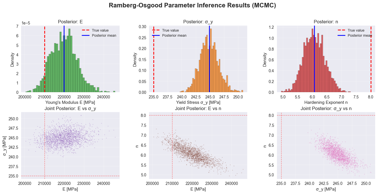
# Create summary statistics
print("\n" + "="*60)
print("POSTERIOR SUMMARY STATISTICS")
print("="*60)
print("Parameter | True Value | Posterior Mean | 95% CI")
print("-"*60)
print(f"E (MPa) | {true_E:10.1f} | {E_samples.mean():14.1f} | [{np.percentile(E_samples, 2.5):.1f}, {np.percentile(E_samples, 97.5):.1f}]")
print(f"σ_y (MPa) | {true_sigma_y:10.1f} | {sigma_y_samples.mean():14.1f} | [{np.percentile(sigma_y_samples, 2.5):.1f}, {np.percentile(sigma_y_samples, 97.5):.1f}]")
print(f"n (hardening exp) | {true_n:10.1f} | {n_samples.mean():14.2f} | [{np.percentile(n_samples, 2.5):.2f}, {np.percentile(n_samples, 97.5):.2f}]")
print("="*60)
# Compute predictive statistics
mean_strain = strain_samples.mean(axis=0)
lower_strain = np.percentile(strain_samples, 2.5, axis=0)
upper_strain = np.percentile(strain_samples, 97.5, axis=0)
fig = plt.figure(figsize=(16, 10))
gs = fig.add_gridspec(3, 3, hspace=0.3, wspace=0.3)
# 1. Loss curve
ax1 = fig.add_subplot(gs[0, 0])
ax1.plot(ro_losses, color="#1f77b4", linewidth=1.5)
ax1.set_xlabel("Iteration")
ax1.set_ylabel("Per-sample ELBO loss")
ax1.set_title("Training Convergence")
ax1.set_yscale("log")
ax1.grid(True, alpha=0.3)
# 2-4. Marginal posteriors
ax2 = fig.add_subplot(gs[0, 1])
ax2.hist(E_samples, bins=50, density=True, color="#2ca02c", alpha=0.7, edgecolor="black")
ax2.axvline(true_E, color="red", linestyle="--", linewidth=2, label="True value")
ax2.axvline(E_samples.mean(), color="blue", linestyle="-", linewidth=2, label="Posterior mean")
ax2.set_xlabel("Young's Modulus E [MPa]")
ax2.set_ylabel("Density")
ax2.set_title("Posterior: E")
ax2.legend(fontsize=9)
ax2.grid(True, alpha=0.3)
ax3 = fig.add_subplot(gs[0, 2])
ax3.hist(sigma_y_samples, bins=50, density=True, color="#ff7f0e", alpha=0.7, edgecolor="black")
ax3.axvline(true_sigma_y, color="red", linestyle="--", linewidth=2, label="True value")
ax3.axvline(sigma_y_samples.mean(), color="blue", linestyle="-", linewidth=2, label="Posterior mean")
ax3.set_xlabel("Yield Stress σ_y [MPa]")
ax3.set_ylabel("Density")
ax3.set_title("Posterior: σ_y")
ax3.legend(fontsize=9)
ax3.grid(True, alpha=0.3)
ax4 = fig.add_subplot(gs[1, 0])
ax4.hist(n_samples, bins=50, density=True, color="#d62728", alpha=0.7, edgecolor="black")
ax4.axvline(true_n, color="red", linestyle="--", linewidth=2, label="True value")
ax4.axvline(n_samples.mean(), color="blue", linestyle="-", linewidth=2, label="Posterior mean")
ax4.set_xlabel("Hardening Exponent n")
ax4.set_ylabel("Density")
ax4.set_title("Posterior: n")
ax4.legend(fontsize=9)
ax4.grid(True, alpha=0.3)
# 5-7. Joint posteriors (2D scatter plots)
ax5 = fig.add_subplot(gs[1, 1])
ax5.scatter(E_samples, sigma_y_samples, s=2, alpha=0.3, color="#9467bd")
ax5.axvline(true_E, color="red", linestyle="--", linewidth=1, alpha=0.5)
ax5.axhline(true_sigma_y, color="red", linestyle="--", linewidth=1, alpha=0.5)
ax5.set_xlabel("E [MPa]")
ax5.set_ylabel("σ_y [MPa]")
ax5.set_title("Joint Posterior: E vs σ_y")
ax5.grid(True, alpha=0.3)
ax6 = fig.add_subplot(gs[1, 2])
ax6.scatter(E_samples, n_samples, s=2, alpha=0.3, color="#8c564b")
ax6.axvline(true_E, color="red", linestyle="--", linewidth=1, alpha=0.5)
ax6.axhline(true_n, color="red", linestyle="--", linewidth=1, alpha=0.5)
ax6.set_xlabel("E [MPa]")
ax6.set_ylabel("n")
ax6.set_title("Joint Posterior: E vs n")
ax6.grid(True, alpha=0.3)
ax7 = fig.add_subplot(gs[2, 0])
ax7.scatter(sigma_y_samples, n_samples, s=2, alpha=0.3, color="#e377c2")
ax7.axvline(true_sigma_y, color="red", linestyle="--", linewidth=1, alpha=0.5)
ax7.axhline(true_n, color="red", linestyle="--", linewidth=1, alpha=0.5)
ax7.set_xlabel("σ_y [MPa]")
ax7.set_ylabel("n")
ax7.set_title("Joint Posterior: σ_y vs n")
ax7.grid(True, alpha=0.3)
# 8. Posterior predictive on stress-strain curve
ax8 = fig.add_subplot(gs[2, 1:])
# Plot observed data
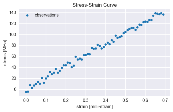
ax8.scatter(strains.numpy() * 1e3, stresses.numpy(),
s=30, color="#1f77b4", alpha=0.6, label="Observed data", zorder=3)
# Plot posterior mean
ax8.plot(mean_strain * 1e3, stresses.numpy(),
color="#2ca02c", linewidth=2.5, label="Posterior mean", zorder=4)
# Plot credible interval
ax8.fill_betweenx(stresses.numpy(), lower_strain * 1e3, upper_strain * 1e3,
color="#2ca02c", alpha=0.2, label="95% credible interval", zorder=1)
ax8.set_xlabel("Strain [milli-strain]")
ax8.set_ylabel("Stress [MPa]")
ax8.set_title("Posterior Predictive: Stress-Strain Curve")
ax8.legend(loc="upper left", fontsize=10)
ax8.grid(True, alpha=0.3)
plt.suptitle("Ramberg-Osgood Parameter Inference Results", fontsize=16, fontweight="bold", y=0.995)
plt.show()