So far, all of the models we have used in this book have assumed that data was given to us, and in many cases fully labeled. However, in many real-world scenarios, obtaining data of any kind (let alone labeled data) can be expensive and time-consuming. Instead, we are often in a position where we can choose what data to collect or label, and we want to make the most of our limited resources. Likewise, we may have access to a large amount of unlabeled data, but labeling it all may be infeasible or too costly. In these situations, we can use techniques from active learning and semi-supervised learning to make the most of the data we can collect.
23.1 Learning Objectives
By the end of this chapter, you will be able to:
Understand the concepts of active learning and semi-supervised learning.
Implement basic active learning strategies, such as Uncertainty sampling, to select informative data points for labeling.
Apply semi-supervised learning techniques, such as label propagation, to leverage unlabeled data in model training.
Evaluate the comparative performance of models trained using active and semi-supervised learning methods on several baseline cases.
23.2 Active Learning
Active learning is a machine learning paradigm where the model can interactively query a user (or some other information source) to obtain the desired outputs for new data points. The main idea is to select the most informative data points to label, thereby maximizing the model’s performance while minimizing the amount of labeled data required. Settles 2010 categorizes active learning approaches into three main settings depending on the type of queries you are able to make:
Membership Query Synthesis: The model can generate new data points and request labels for them. This is often used in scenarios where the model can create synthetic examples. Common examples that would occur in Engineering include:
Running simulations with specific input parameters and querying the output. For example, running a CFD simulation with a given geometry or boundary condition. In these cases, I can choose which samples/datapoints I want to run the simulation for and can decide at any time to generate new or different ones.
Conducting experiments with specific configurations and querying the results. For example, in a materials science context, I might choose to synthesize a material with certain properties and then measure its performance.
Stream-based Selective Sampling: The model receives a stream of unlabeled data points and must decide whether to query the label for each point as it arrives. This is common in scenarios where data arrives in real-time, such as:
Monitoring sensor data from an IoT device (e.g., a video or audio sensor on a production line or mobile robot) and deciding whether to request human annotation for specific readings that are uncertain or unusual.
Analyzing streams of incoming user interactions on a website or device and choosing to label certain actions (e.g., clicks, purchases, motions) based on their potential informativeness for improving your prediction system.
Pool-based Sampling: The model has access to a large pool of unlabeled data and can select specific points from this pool to query for labels. This is common in engineering scenarios where a large dataset is available, but labeling is expensive, such as:
Selecting parts from a production run to inspect or possibly perform destructive testing on, in order to improve a quality control model.
You can synthesize a large number of design variations (e.g., different geometries, materials, or configurations) and then select a subset to simulate or test in order to improve a predictive model for performance or reliability. For example, if you have a manufacturing process parameter that can produce a variety of randomized material microstructures (e.g., metal foams with various pore sizes and distributions), you might generate a large pool of these microstructures and then select only a few to experimentally test in order to improve your model for predicting mechanical properties.
Depending on your use case, one of these settings may be more appropriate than the others, and the below algorithms may need to be adapted accordingly. In addition, you may need to consider whether you sample data sequentially (i.e., one at a time, updating your model after each new label) or in batches (i.e., selecting multiple data points to label at once before updating your model). The latter is reffered to as batch-mode active learning and is often more practical in real-world scenarios where labeling multiple data points at once is more efficient. For example, the setup costs for a metal powder-bed laser fusion test may be high, so it makes sense to run multiple parts in one go rather than setting up the machine for each individual test. In these cases, we need to consider not only the value of a given datapoint, but rather the value of a set of datapoints.
23.3 Types of Active Learning Strategies
There are several strategies for selecting which data points to label in active learning. The most common general strategies (outlined in Settles 2010) include:
Uncertainty Sampling: The model selects data points for which it is least certain about the predicted label. The advantage of this approach is that it focuses on the areas of the input space where the model is most unsure, which can lead to significant improvements in performance with fewer labeled examples. It is also often relatively simple to implement. The main disadvantage is that it may focus too much on outliers or noisy data points, which can lead to suboptimal performance, and also the points where the model is most uncertain may not always be the most informative for improving the model. Specific common uncertainty measures are:
Least Confidence: Select the data point with the lowest predicted probability for the most likely class.
Margin Sampling: Select the data point with the smallest difference between the top two predicted class probabilities.
Entropy-based Sampling: Select the data point with the highest entropy in the predicted class probabilities.
Query-by-Committee: A committee of models is trained on the current labeled data, and data points are selected based on the disagreement among the committee members. The idea is that if different models disagree on a data point, it is likely to be informative. The advantage of this approach is that it can work across a wide variety of model types, since all one has to compute is the final decision of each model in the committee. The disadvantage is that it can be computationally expensive to train multiple models, and the choice of committee members can significantly impact performance.
Expected Model Change: Data points are selected based on the expected change in the model parameters if the point were to be labeled and added to the training set. This approach aims to select points that will have the most significant impact on the model. The main advantage of this approach is that it directly targets points that will change the model, potentially leading to faster learning compared to, say, uncertainty sampling. The disadvantage is that it can be computationally intensive, as it requires estimating the impact of each potential data point on the model parameters. In the general case, this could mean retraining the model for each candidate point, which is often infeasible. However, for certain models (e.g., linear models), efficient approximations can be used that make this approach more practical.
Expected Error Reduction: Data points are selected based on the expected reduction in the model’s generalization error if the point were to be labeled and added to the training set. This approach aims to select points that will most improve the model’s performance on unseen data. This is in some sense the most “natural” metric of performance with which to select new datapoints, and thus the main advantage of this approach is that it directly targets points that will improve the model’s performance on unseen data. The disadvantage is that it can be computationally intensive, as it requires estimating the impact of each potential data point on the model’s generalization error. This often involves not only retraining the model multiple times, but also then testing it on a held-out validation set. This can become infeasible for complex models or large datasets. However, for certain models (e.g., Gaussian processes), efficient approximations can be used that make this approach more practical.
Variance Reduction: Data points are selected based on the expected reduction in the model’s output variance if the point were to be labeled and added to the training set. This approach aims to select points that will directly reduce the uncertainty in the model’s predictions. The advantage of this approach is that it can lead to more confident predictions, which can be particularly useful in scenarios where uncertainty quantification is important. It is also often the case that data points that are most useful for reducing the model’s variance are not necessarily those points about which the model is most uncertain. The disadvantage is that it can be computationally intensive, as it requires estimating the impact of each potential data point on the model’s output variance, which may not be easily computable compared to, say, a decision surface or likelihood. However, for certain models (e.g., Gaussian processes), efficient approximations can be used that make this approach more practical.
Density-Weighted Methods: These methods take into account the distribution of the unlabeled data when selecting points to label. The idea is to prefer points that are not only uncertain but also representative of the overall data distribution. The advantage of this approach is that it can help avoid selecting outliers or noisy points that may not be representative of the underlying data distribution. The disadvantage is that it can be more complex to implement, as it requires estimating the density of the unlabeled data, which can be challenging or have large numerical variance in high-dimensional spaces.
For this chapter, we will focus only on implementing Uncertainty Sampling due to its relative simplicity and wide applicability in many practical scenarios.
In the example below, we will use a Gaussian Process regression model to select data points to label based on uncertainty sampling. At a high level, a Gaussian Process (GP) is a non-parametric model that defines a distribution over functions. It is particularly well-suited for active learning because it provides not only predictions but also uncertainty estimates for those predictions. Specifically, the mean and variance of the GP’s predictions can be expressed in the following closed-form equations:
\(\mu(x_*)\) is the predicted mean at the new input point \(x_*\).
\(\sigma^2(x_*)\) is the predicted variance at the new input point \(x_*\).
\(k(x_*, X)\) is the covariance vector between the new input point \(x_*\) and the training inputs \(X\).
\(K(X, X)\) is the covariance matrix of the training inputs.
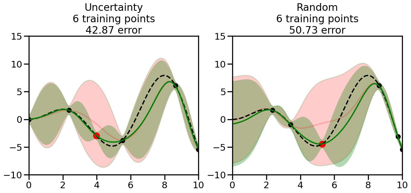
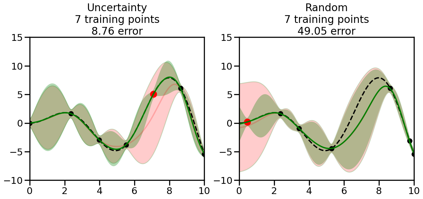
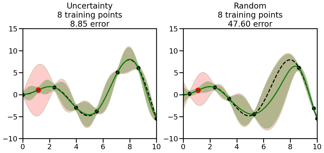
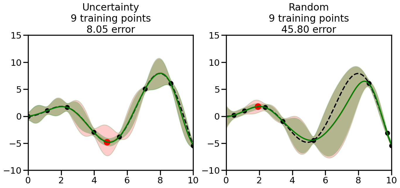
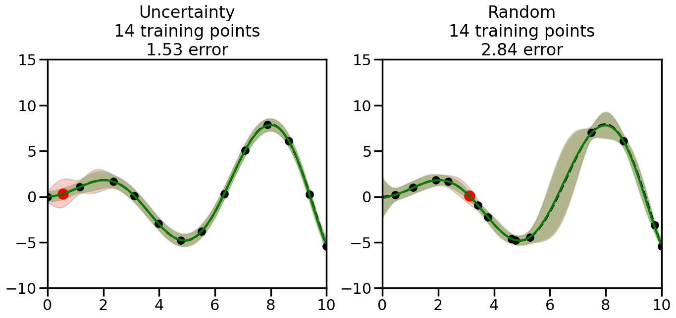
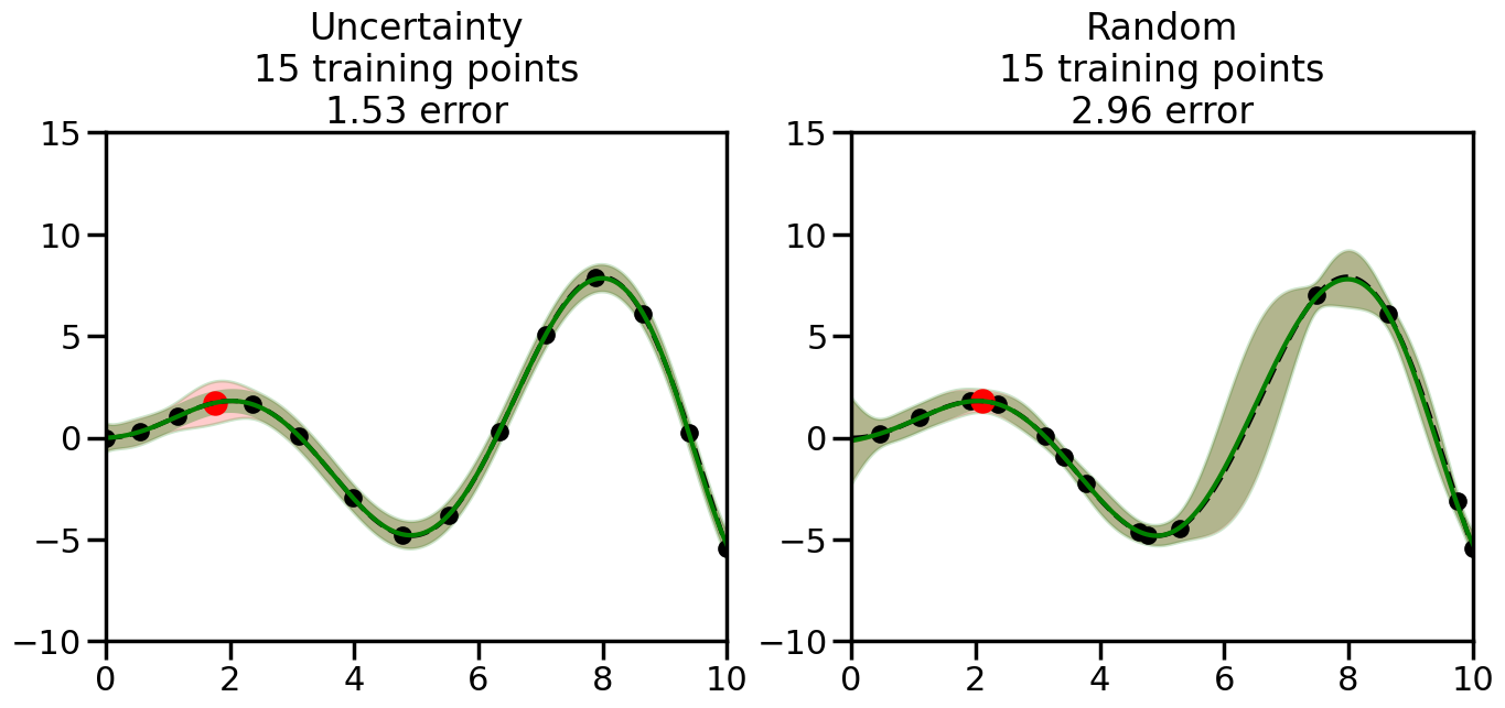
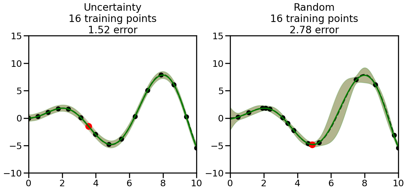
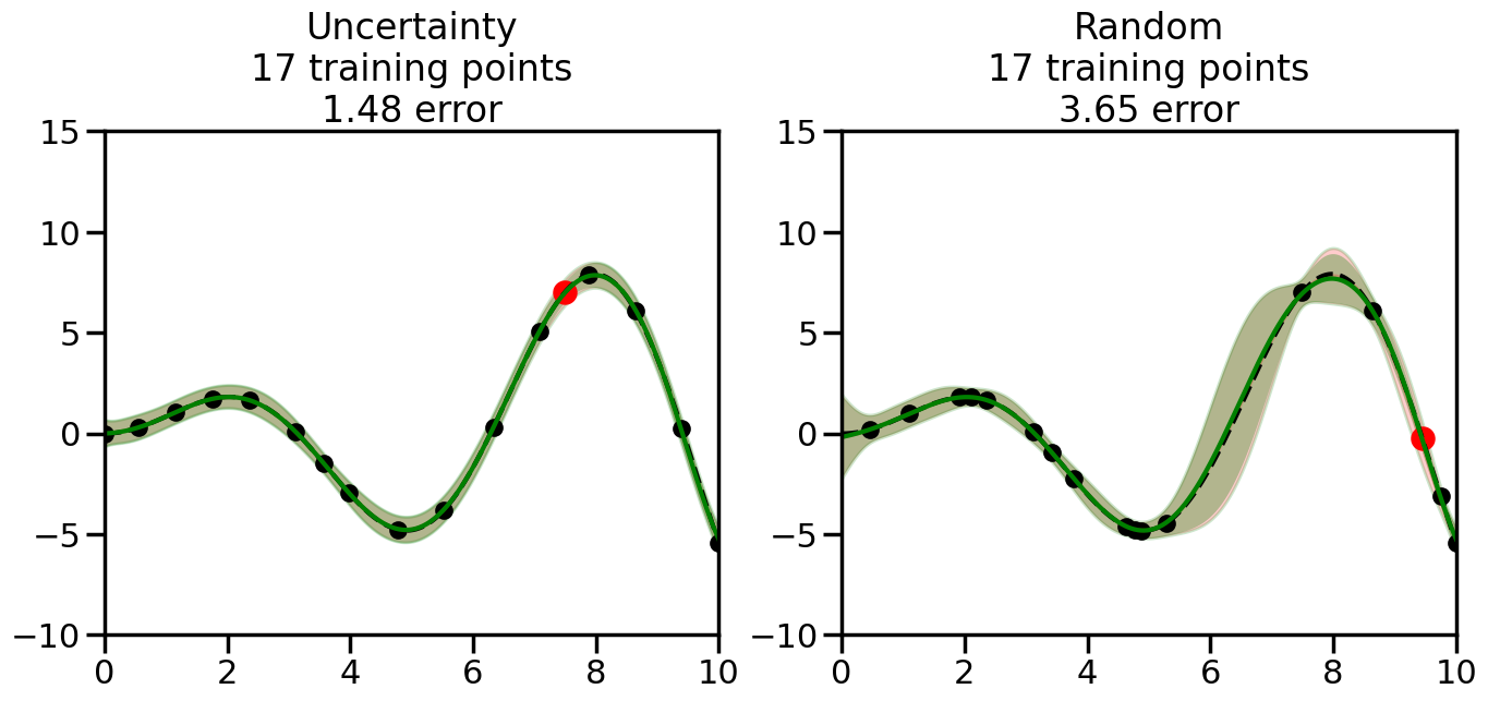
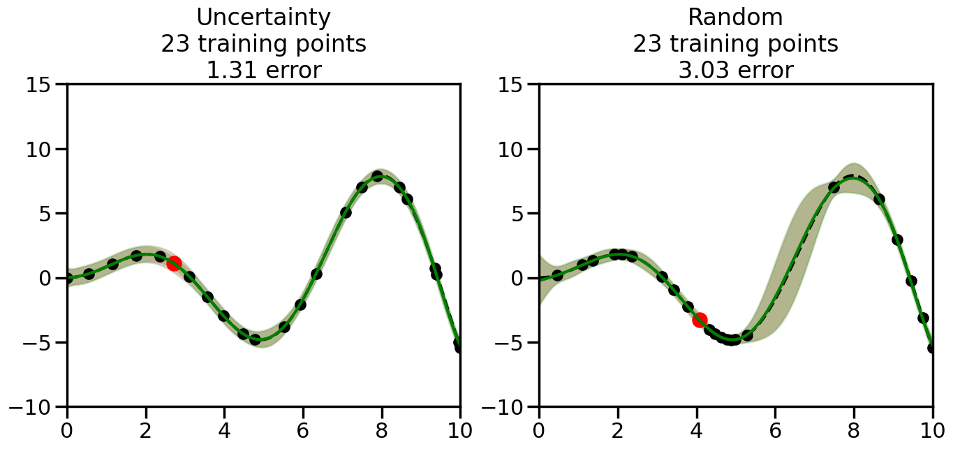
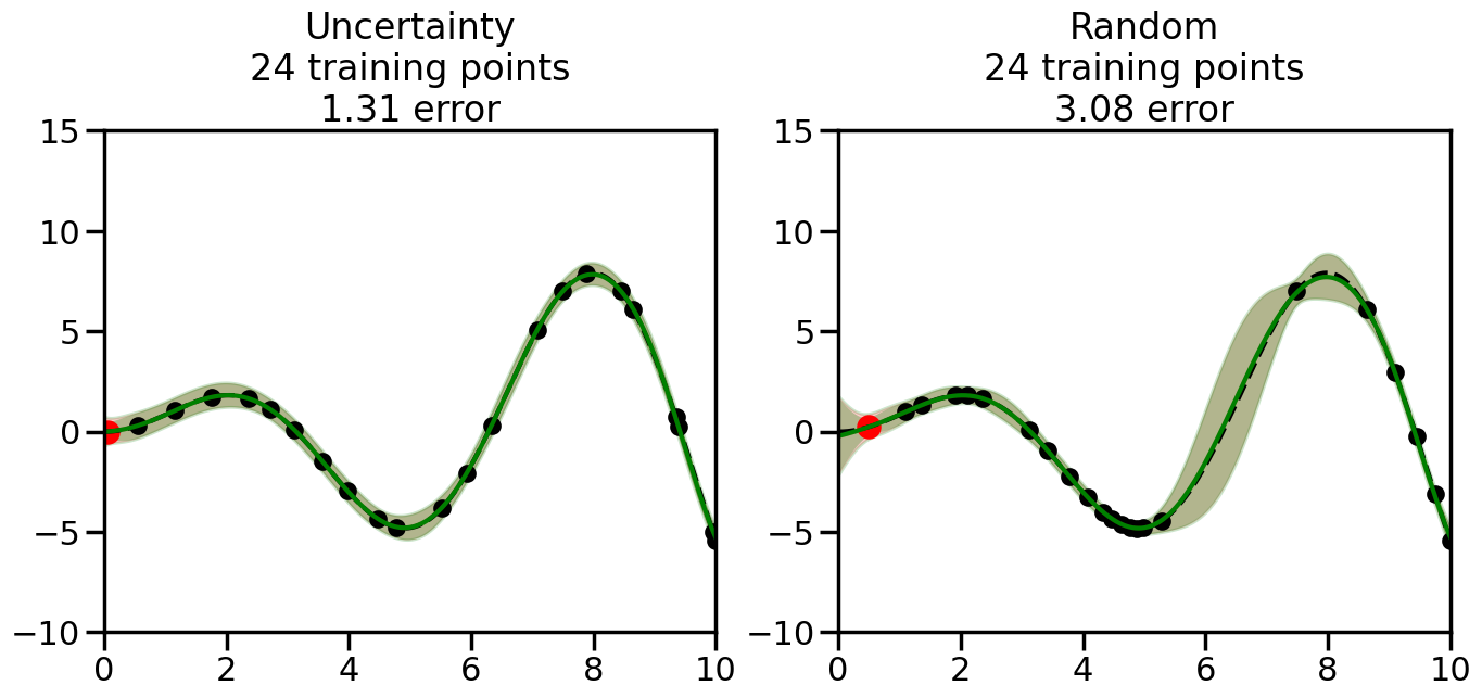
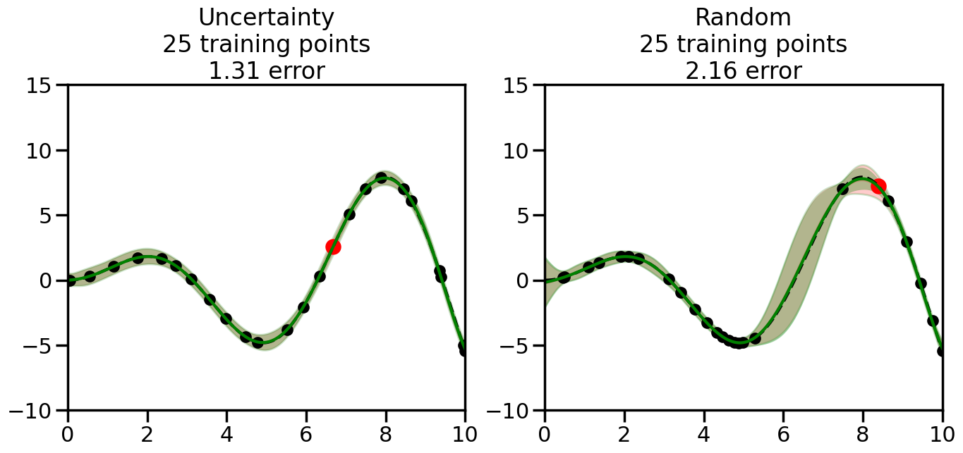
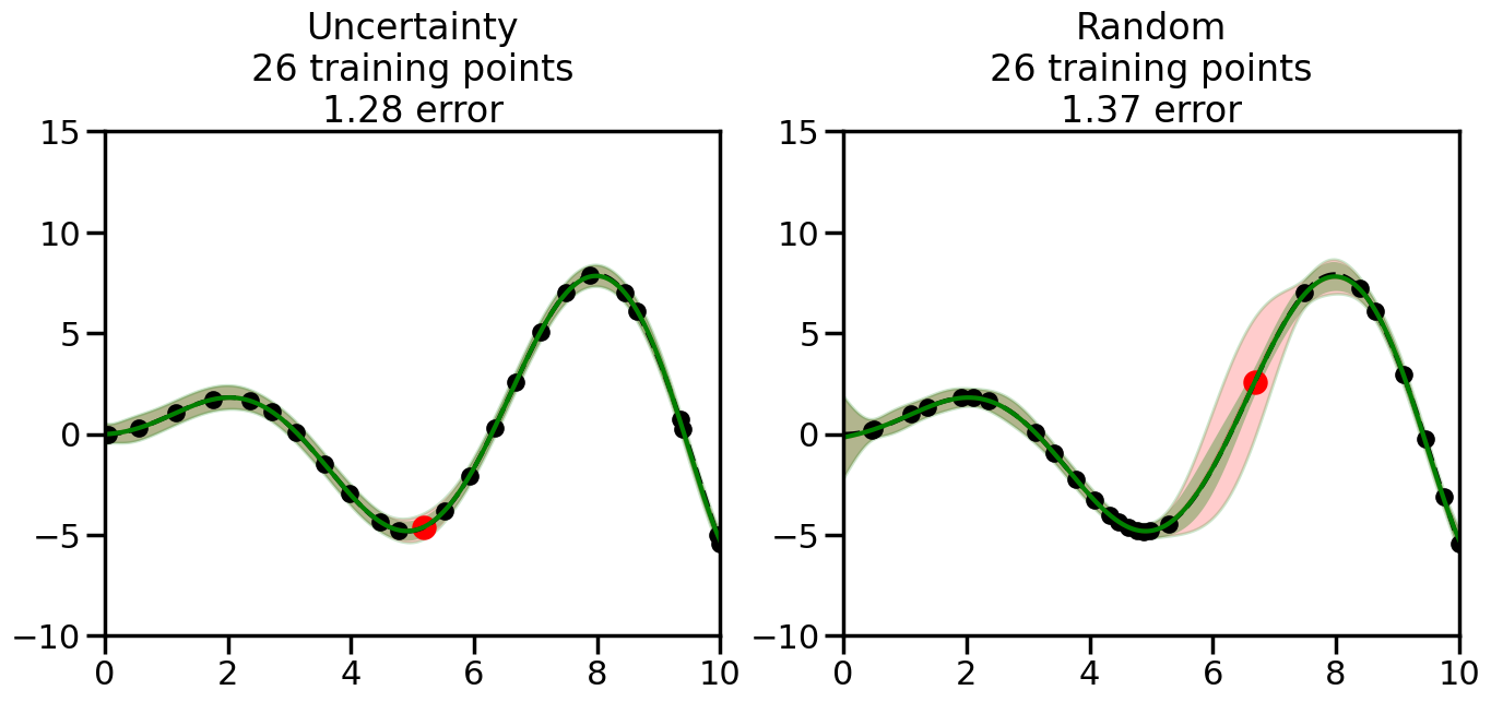
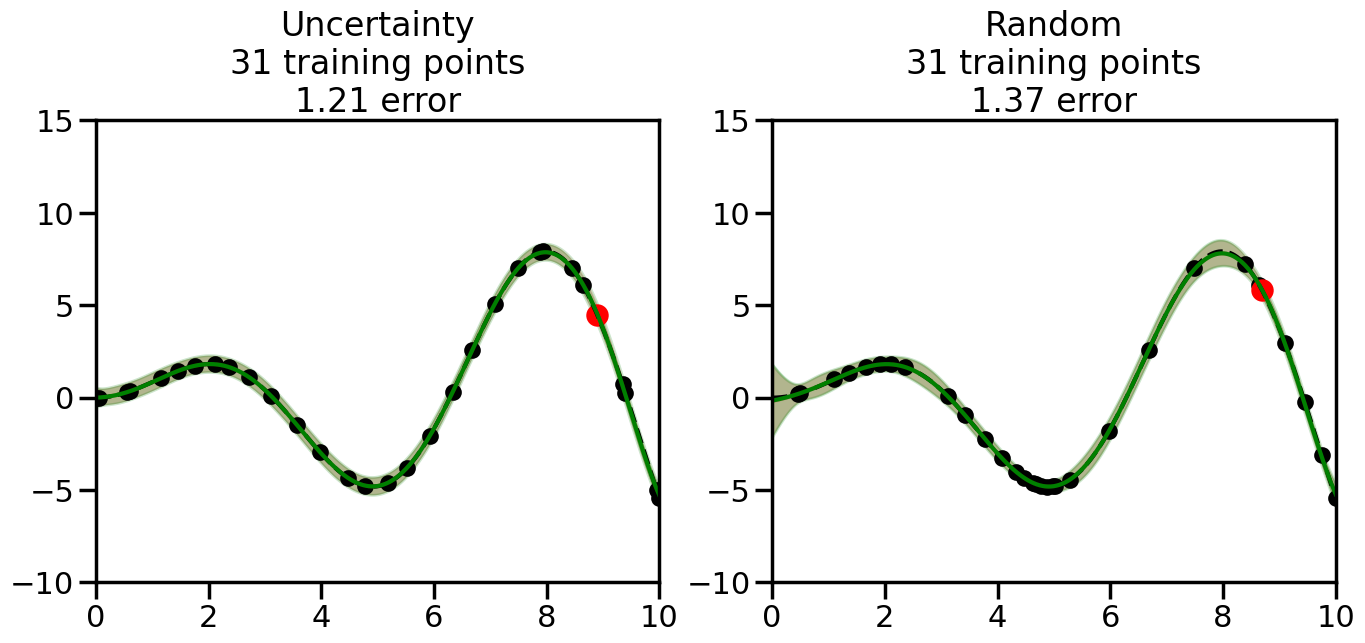
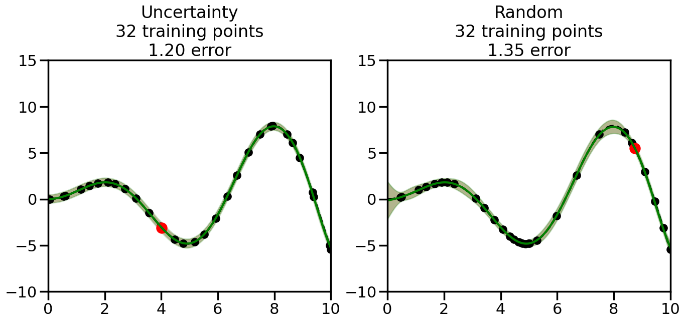
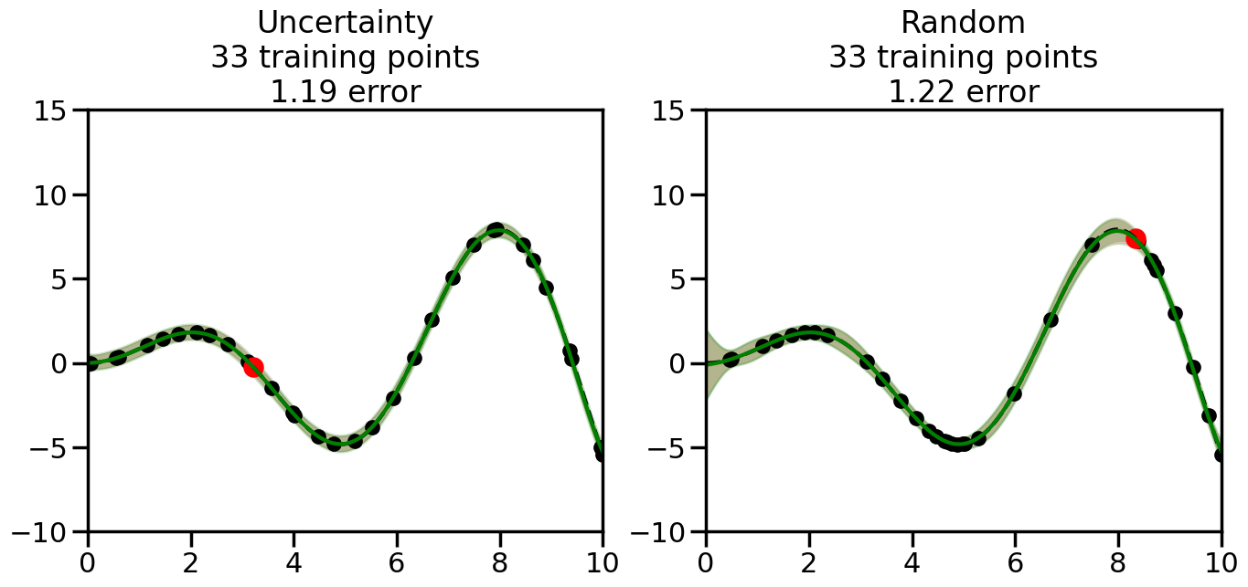
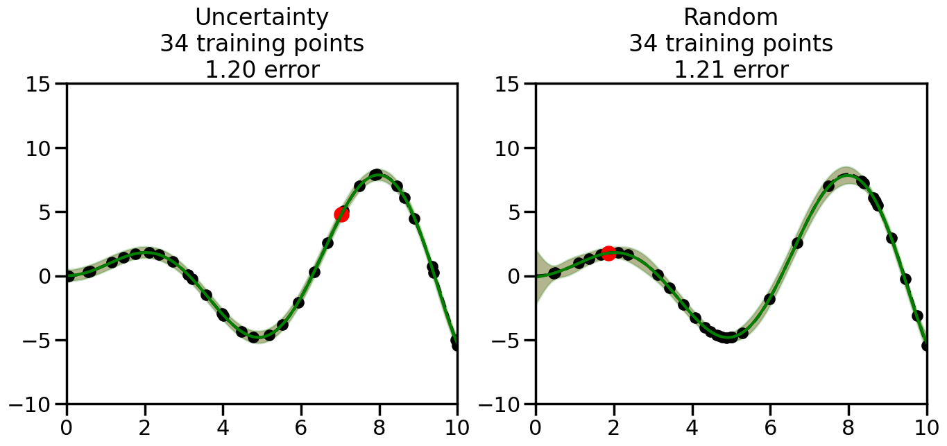
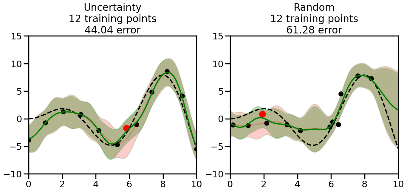
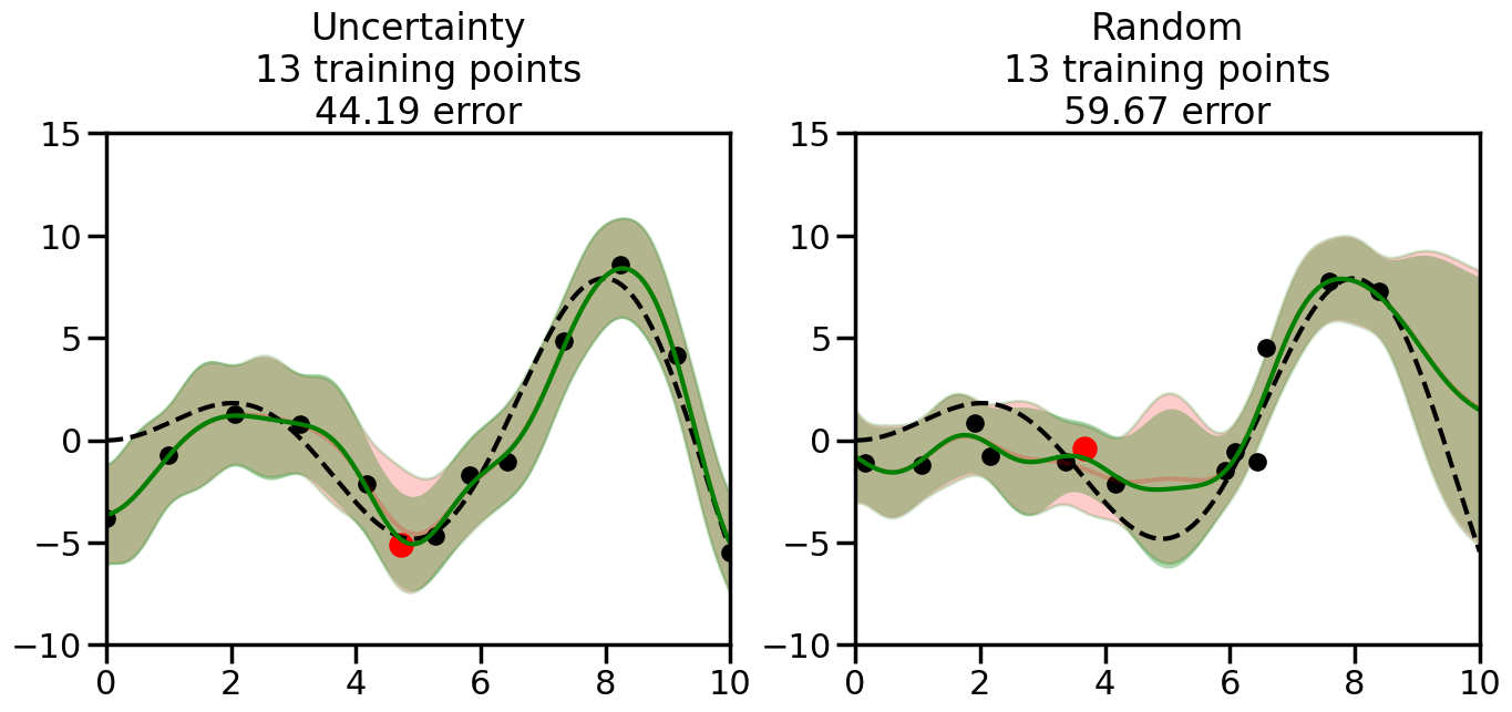
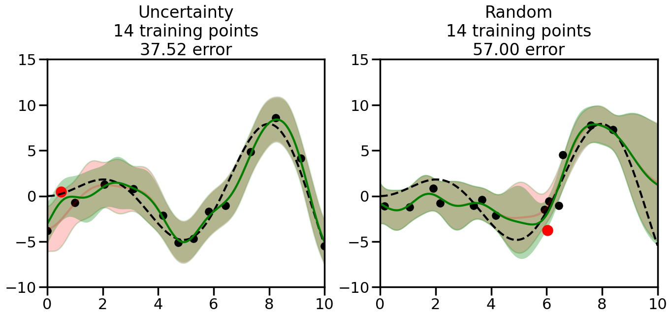
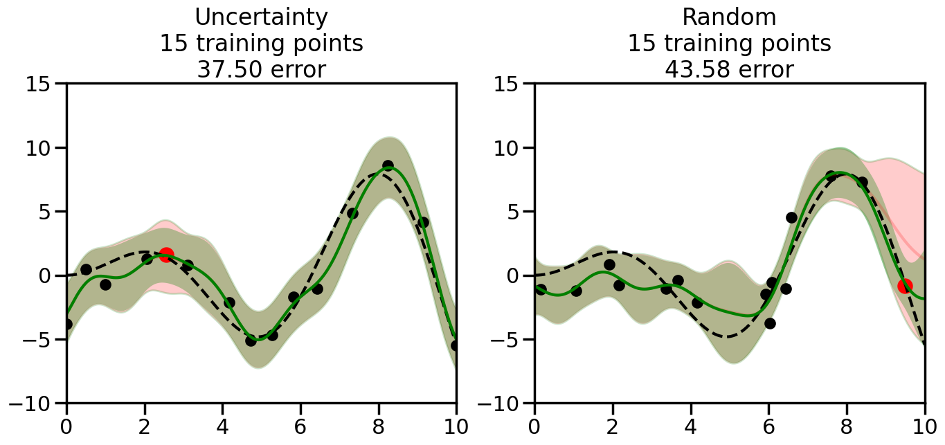
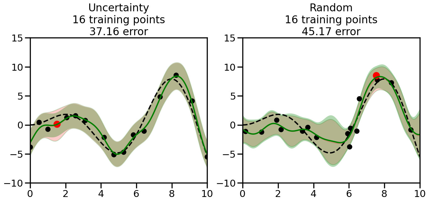
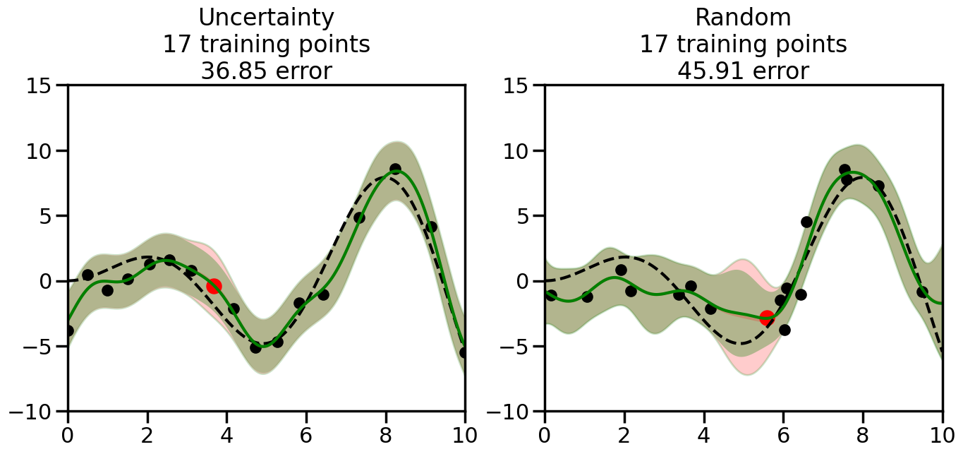
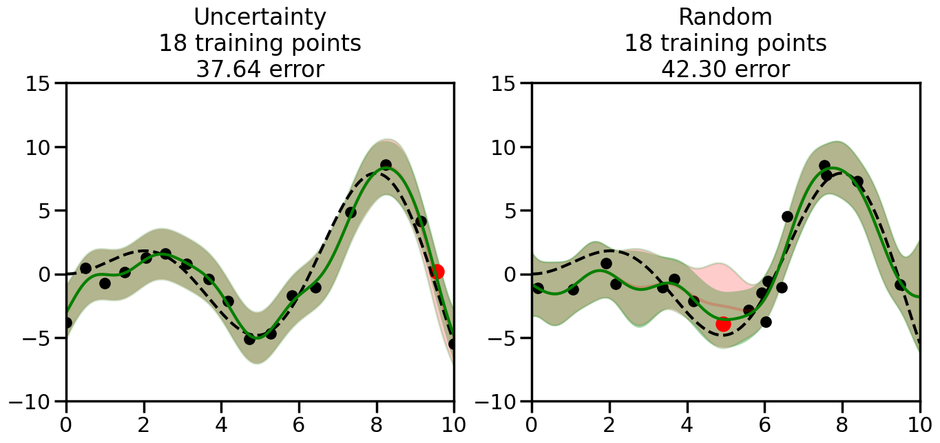
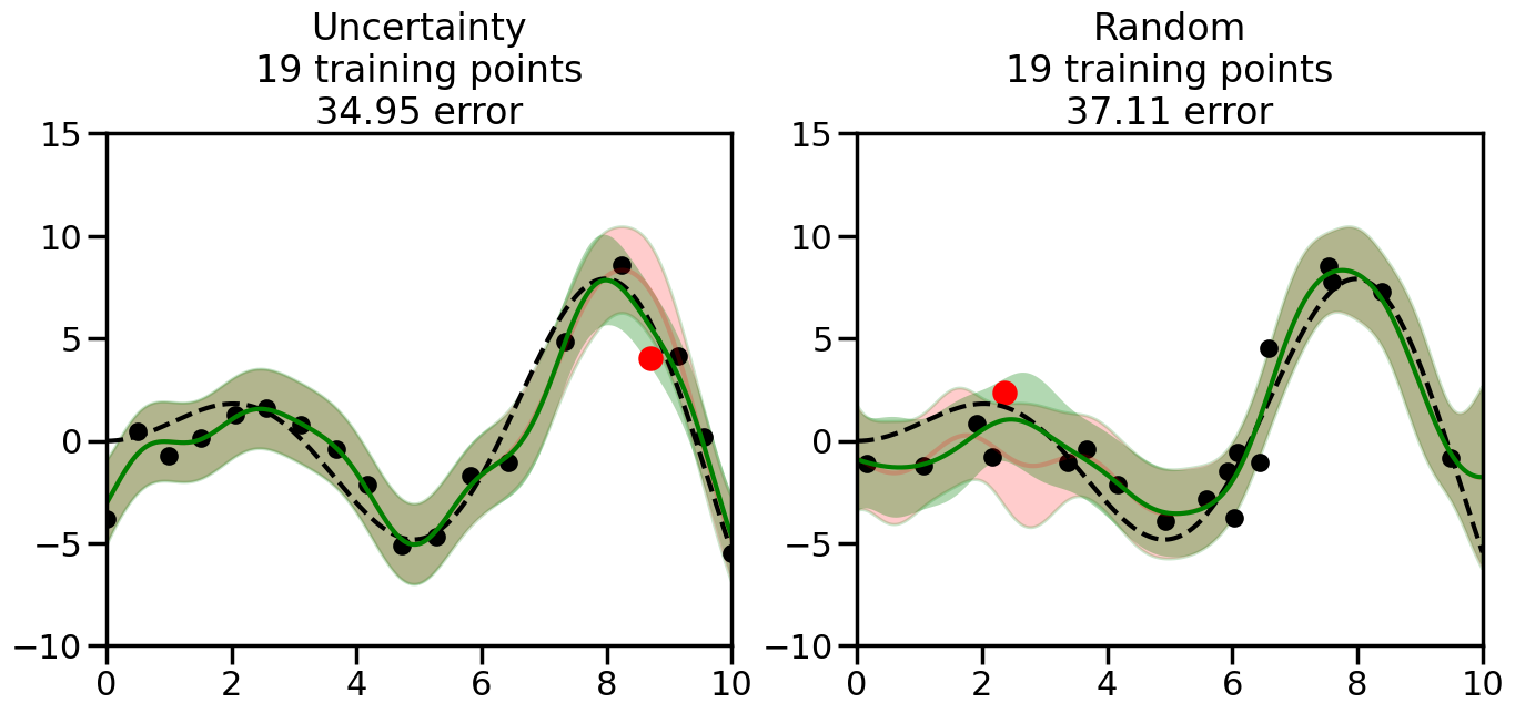
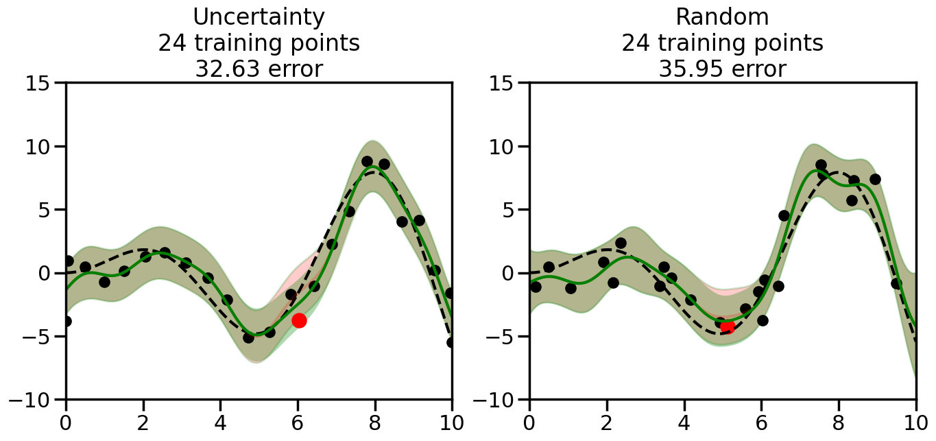
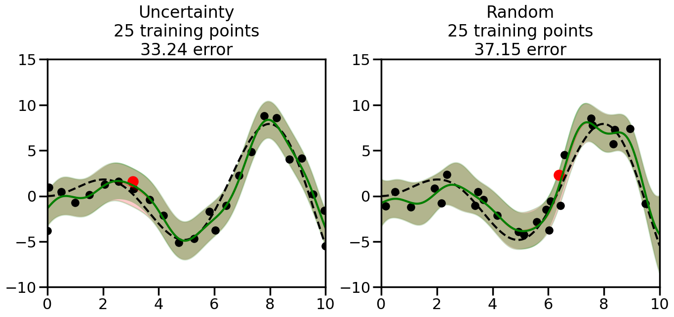
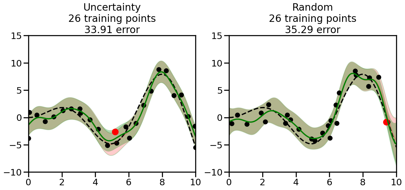
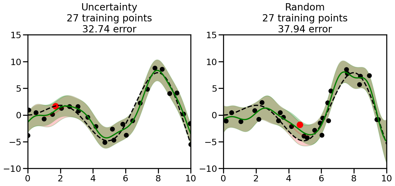
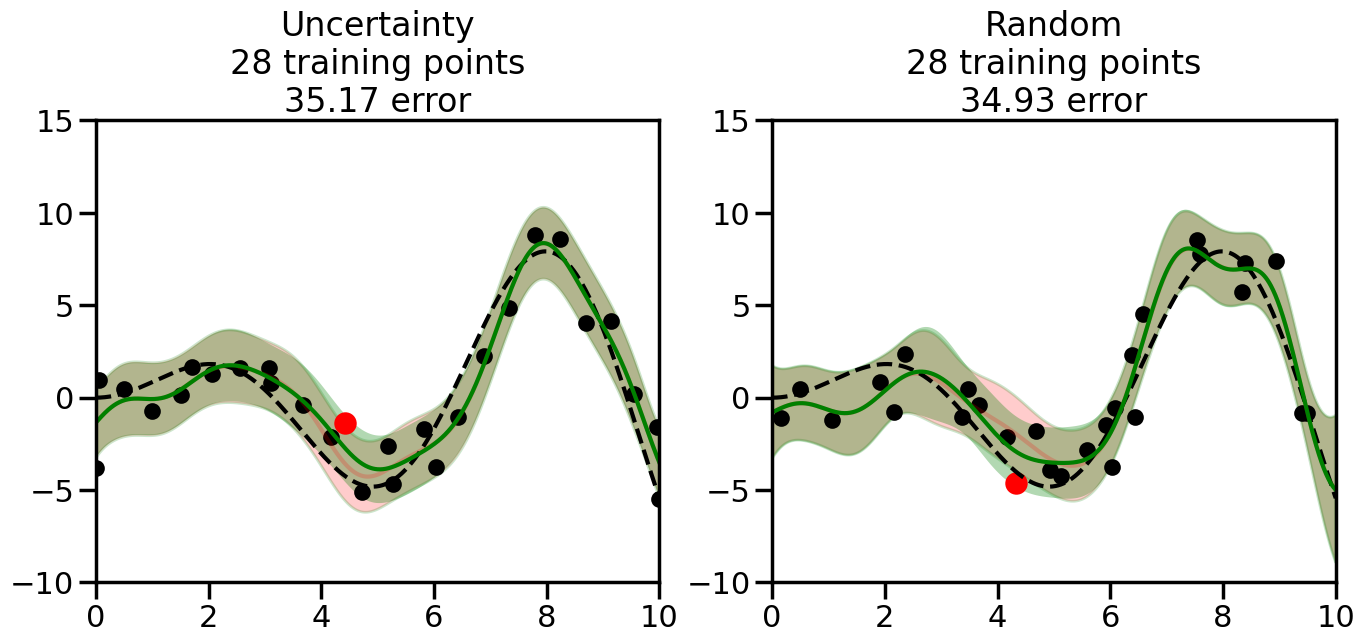
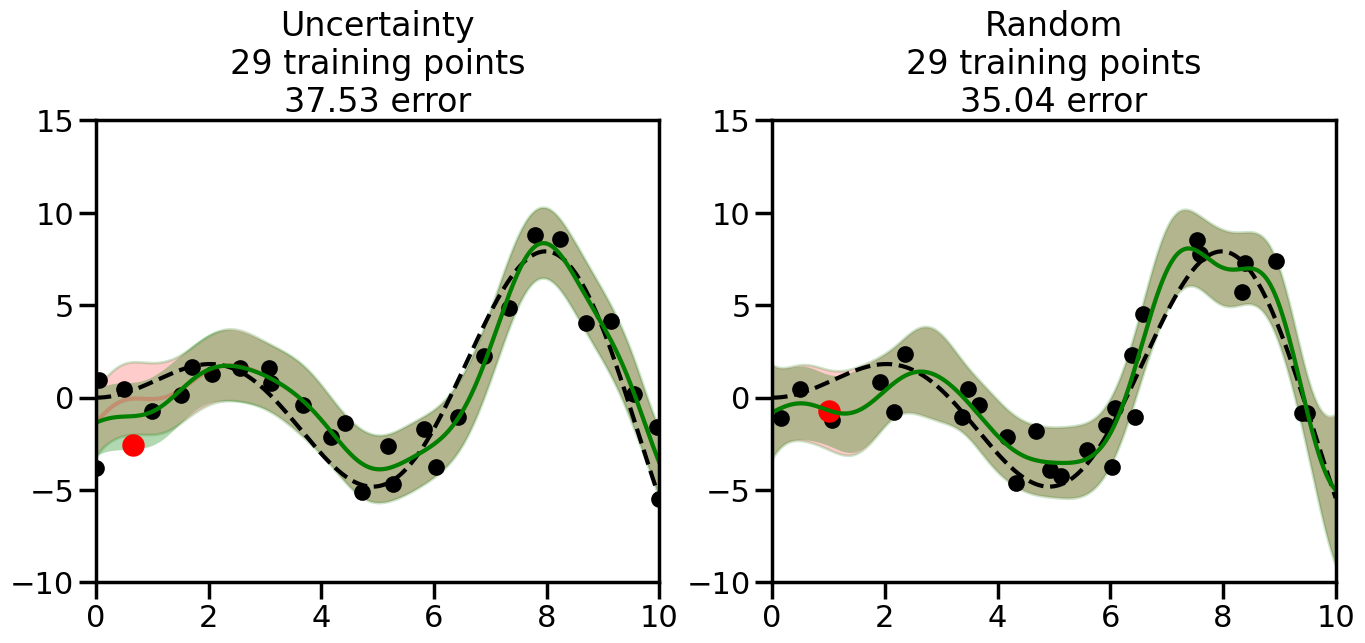
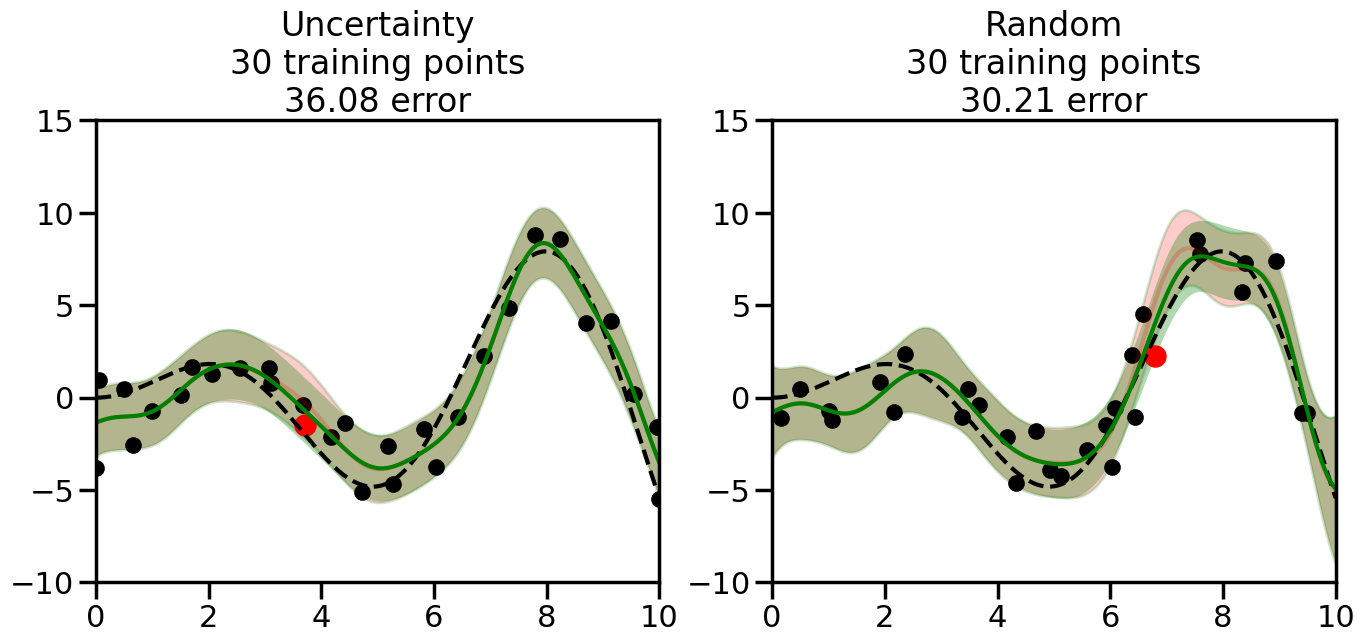
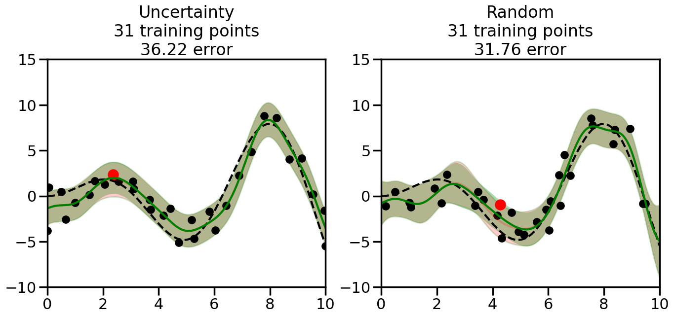
We can see from the above that the uncertainty of the model’s predictions is directly given by the predicted variance \(\sigma^2(x_*)\). Thus, in uncertainty sampling, we can just test the model on several candidate \(x\) locations that we haven’t yet measured and select the data points with the highest predicted variance for labeling. Below we will create a sample “true” function (the dashed line), and then generate noisy observations of this function at a few initial points. We will then iteratively select new points to label based on uncertainty sampling and update our GP model accordingly. For comparison sakes, we will also implement a random sampling strategy where new points are selected randomly from the pool of unlabeled data.
Code
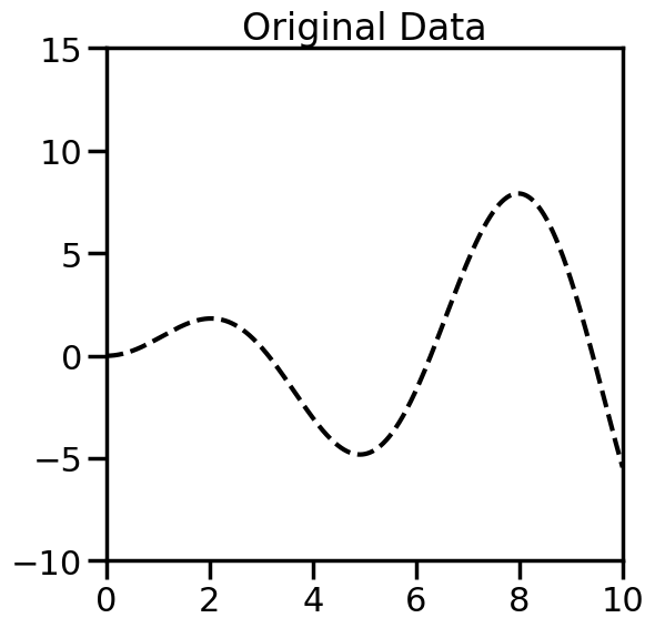
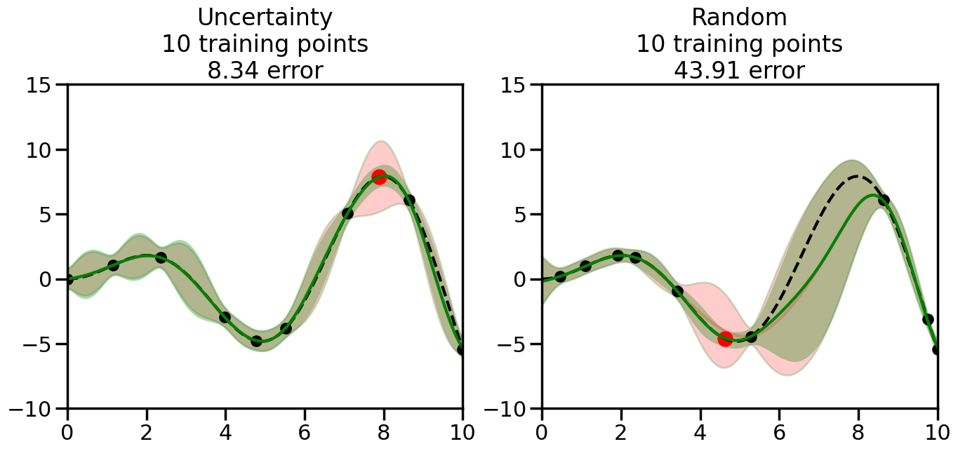
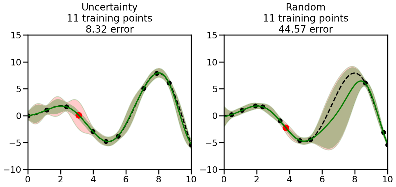
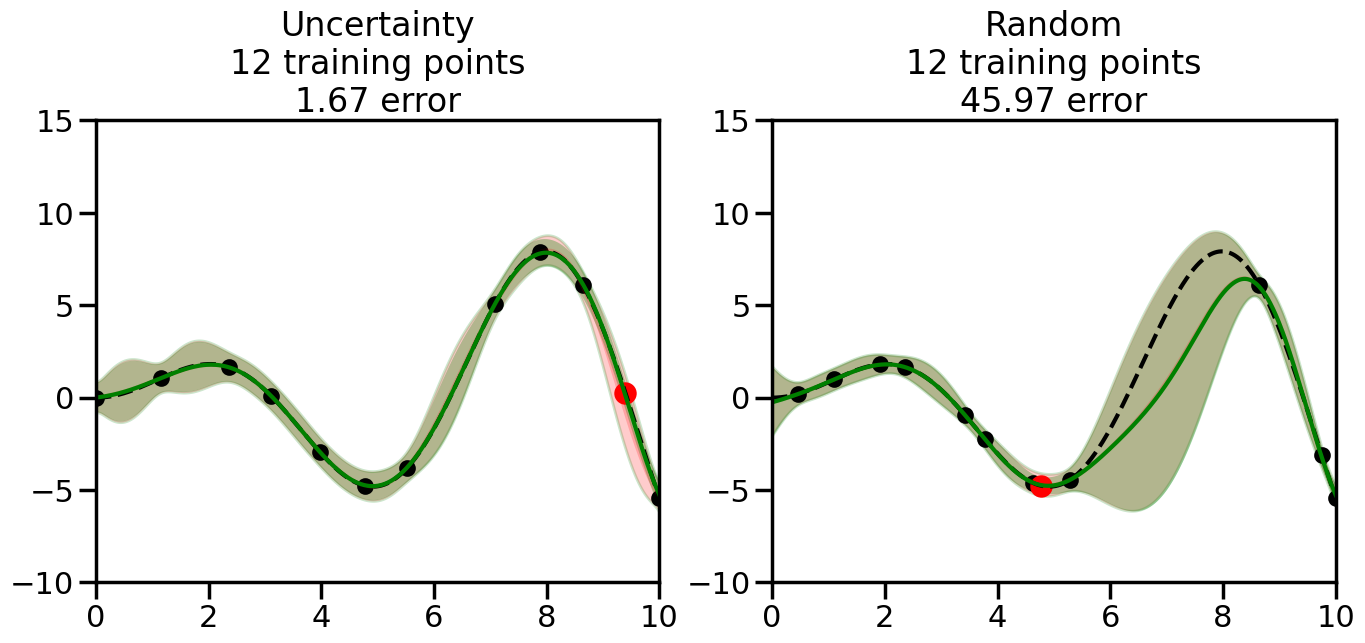
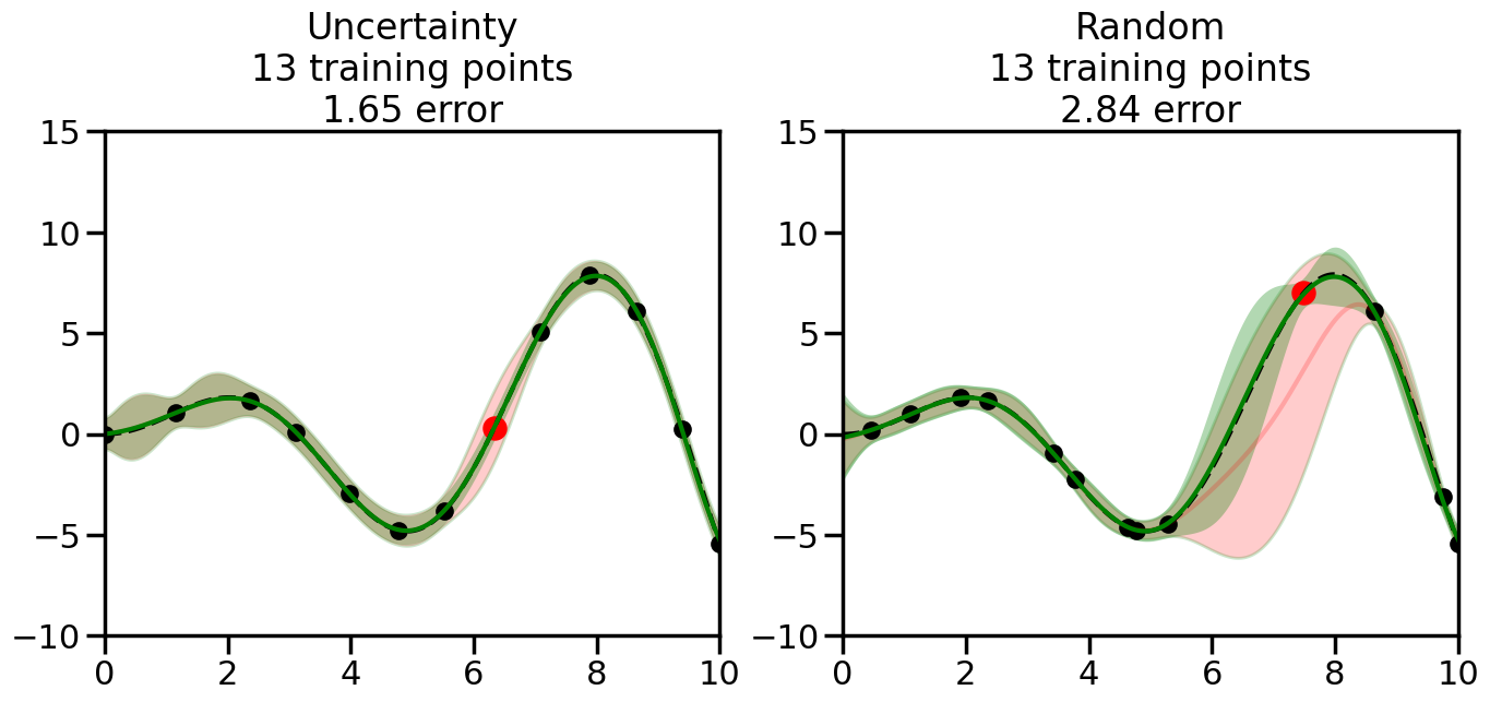
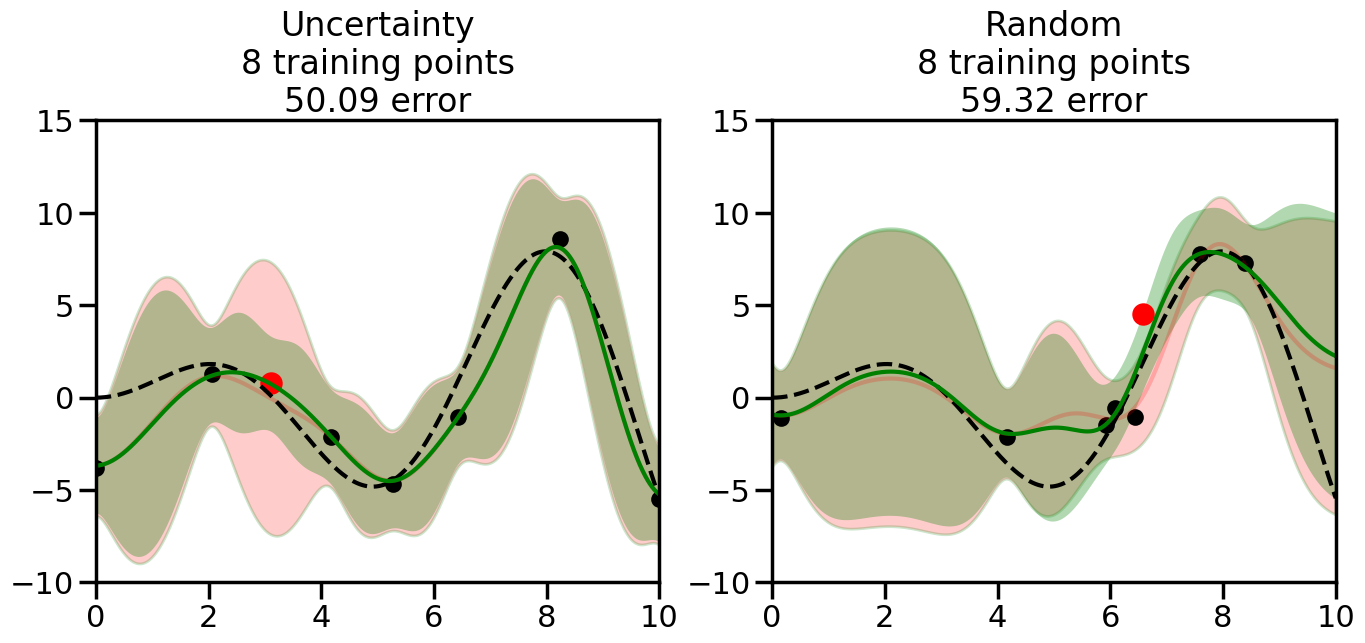
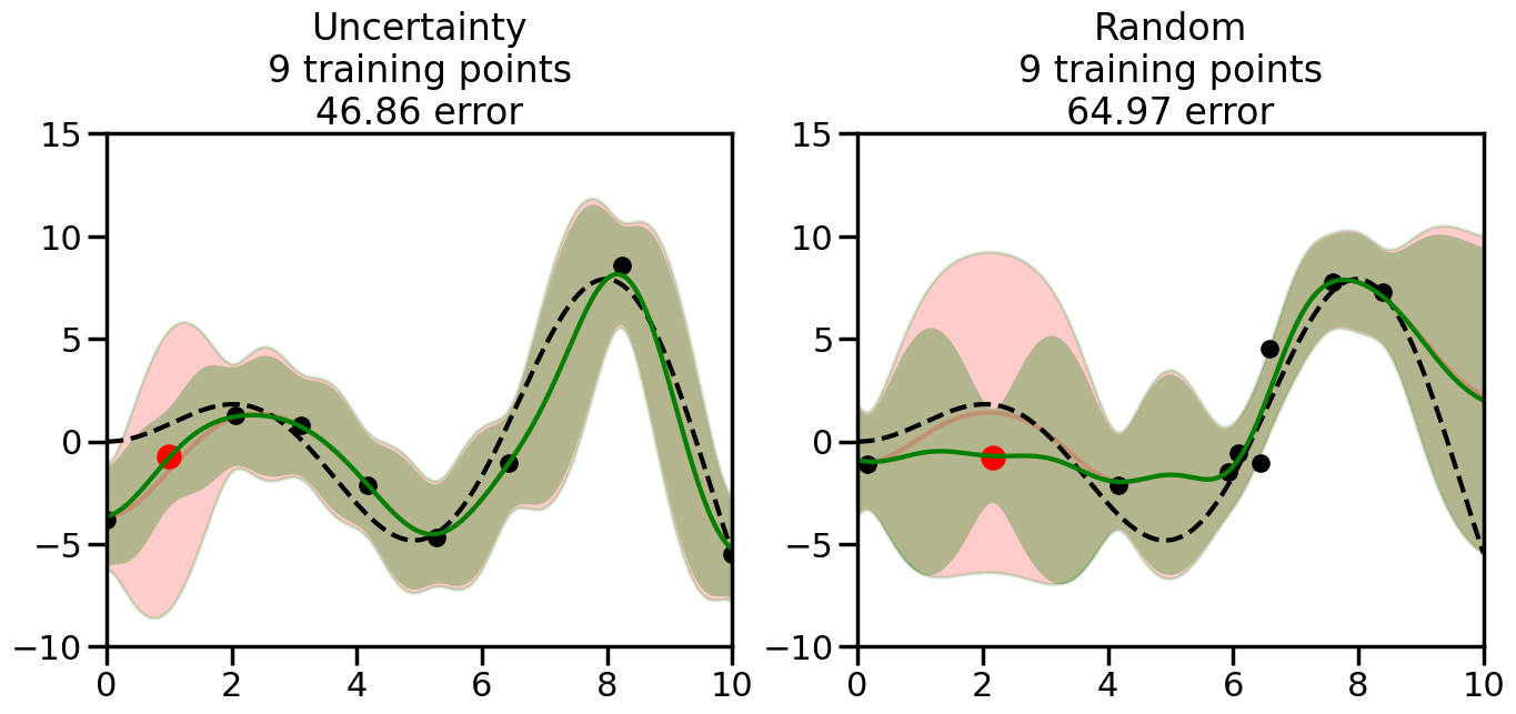
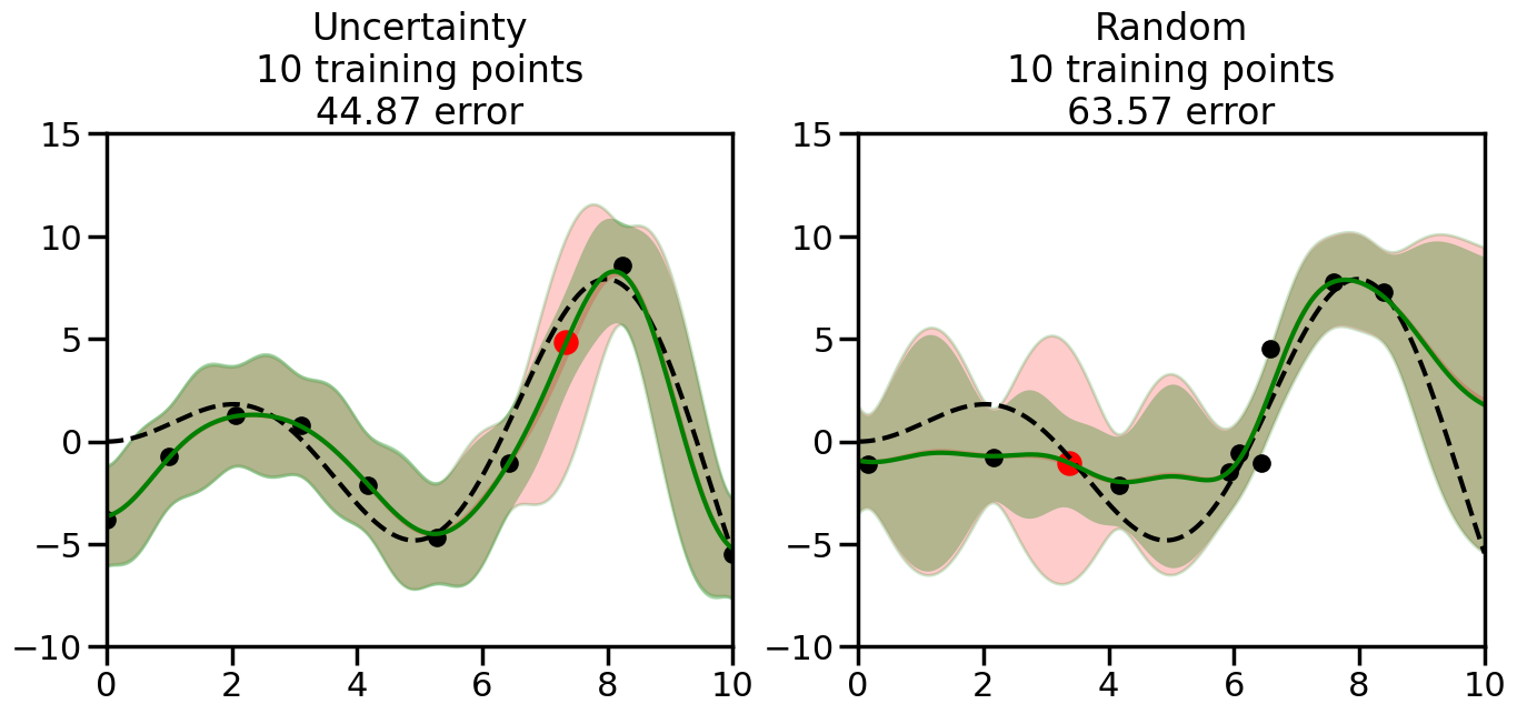
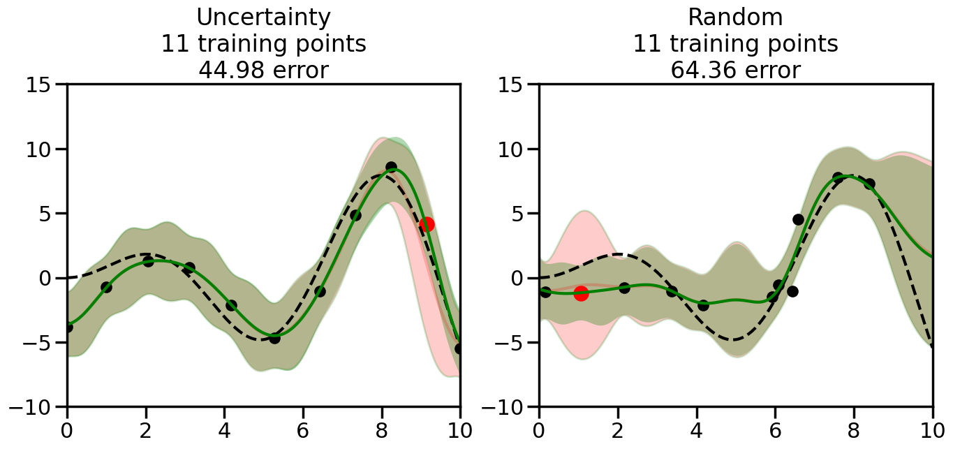
import numpy as npimport matplotlib.pyplot as pltimport seaborn as snssns.set_context('poster')from sklearn.gaussian_process import GaussianProcessRegressor, GaussianProcessClassifierfrom sklearn.gaussian_process.kernels import RBF, WhiteKernel, RationalQuadratic, ExpSineSquared, Maternfrom sklearn.semi_supervised import LabelSpreadingnp.random.seed(0) # Set random seed so that we see the same thing# Define a function to generate samples# Feel free to add your own or change thingsdef f(x):"""The function to predict."""return x * np.sin(x)# Try others!#return 5 * np.sinc(x)#return x# This generates points we will pick from during the active learningX = np.atleast_2d(np.linspace(0, 10, 200)).T# Observations at each of the possible points# (We will only observe a subset of these)y = f(X).ravel()# Generate points for plotting the predicted functionx = np.atleast_2d(np.linspace(0, 10, 1000)).Tplt.figure(figsize=(6,6))# Plot the original functionplt.plot(x,f(x),'k--',alpha=1)plt.ylim([-10,15]) # Set the y-axis limitsplt.xlim([0,10]) # Set the x-axis limitsplt.title("Original Data")plt.show()
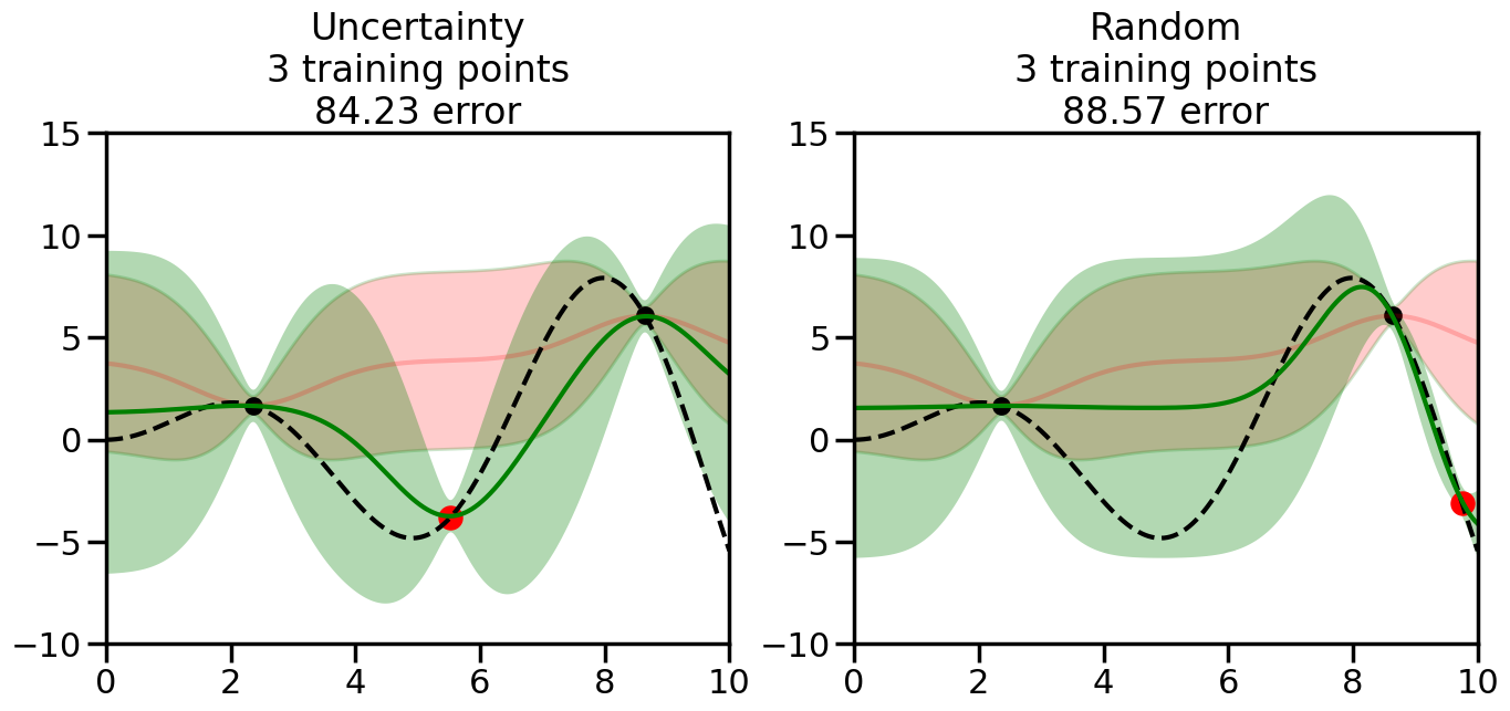
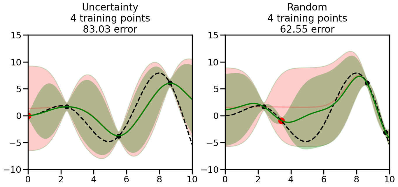
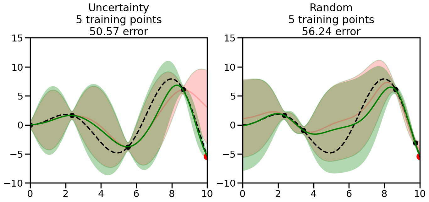
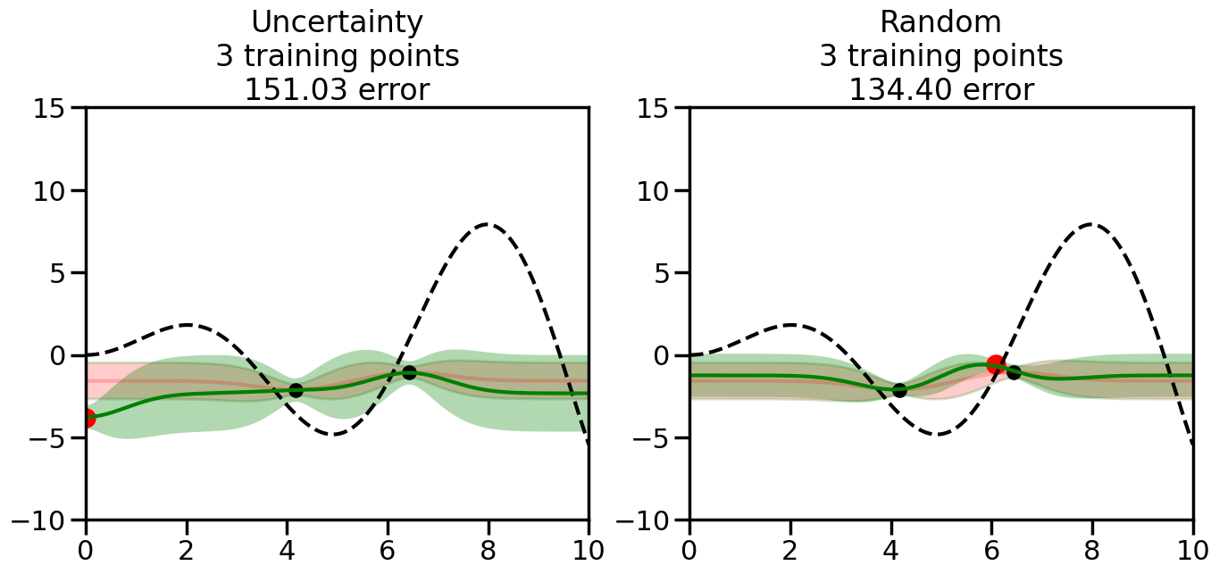
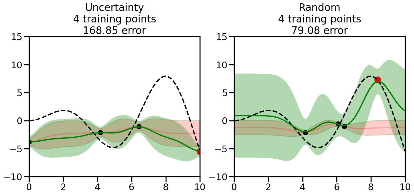
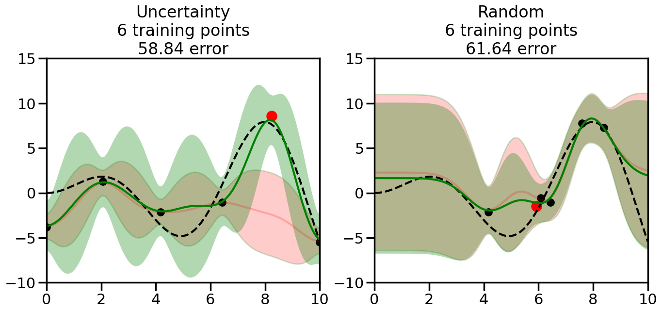
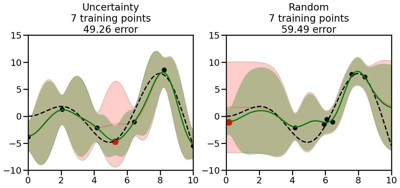
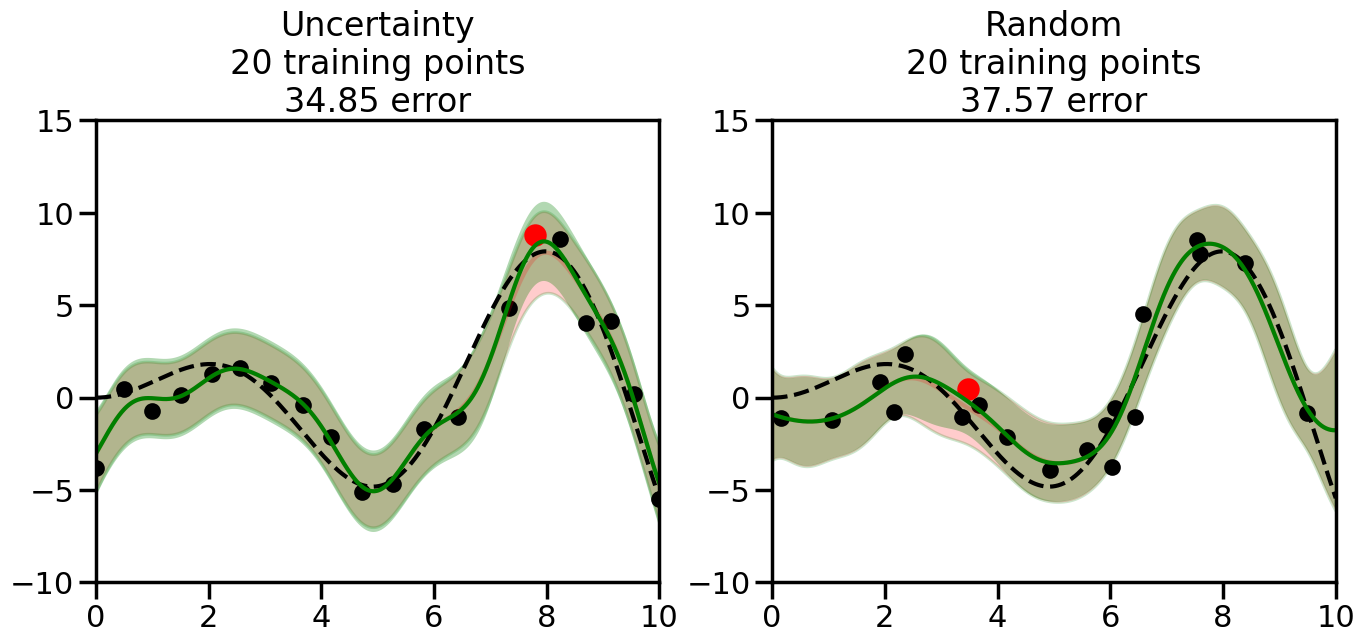
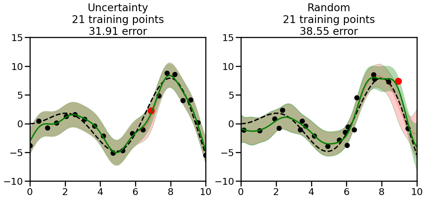
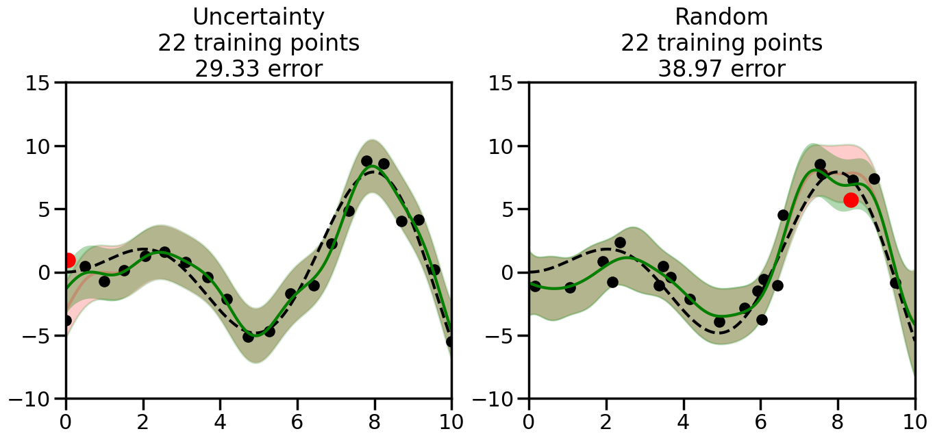
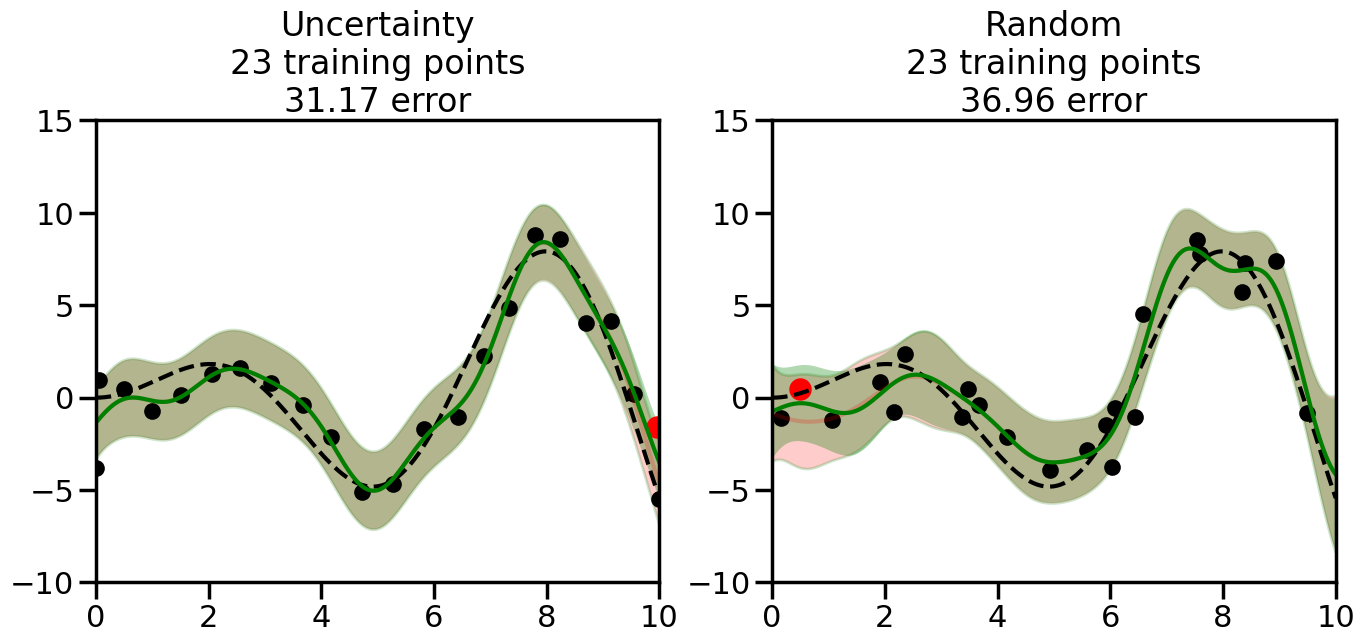
We will now create a Gaussian Process model and implement the uncertainty sampling strategy. For this, we will need to pick a kernel function for the GP, which we will choose to be the Radial Basis Function (RBF) kernel for this example. (However, you can modify the code cell below if you want to experiment with other kernel functions.) In addition, we will need to decide on the number and placement of the initial labeled data points, since otherwise the model will have no information to start with. Common strategies here include random sampling, Latin Hypercube Sampling, or selecting points that are evenly spaced (or at the boundaries of) the input space. For simplicity, we will use random sampling for the initial points in this example, although you can modify the code cell below to experiment with other strategies if you wish.
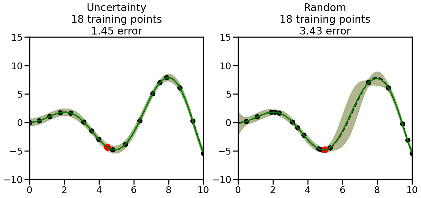
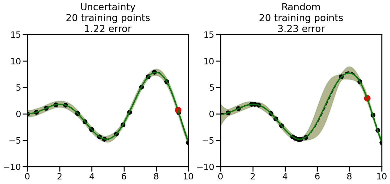
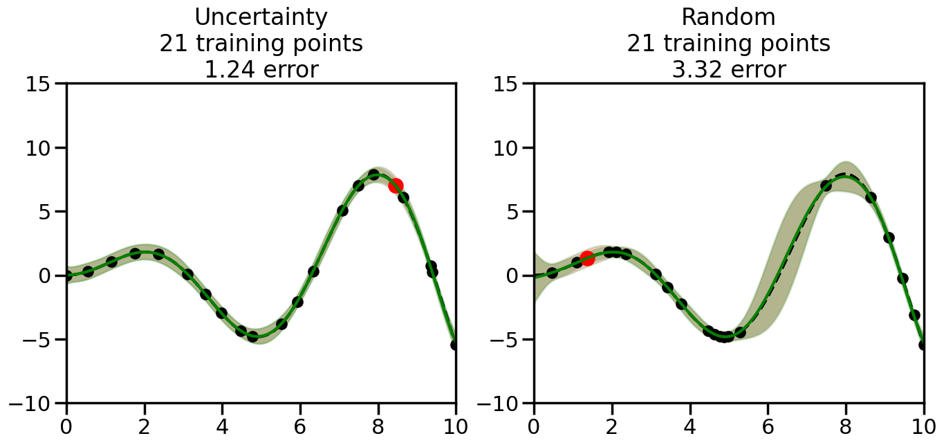
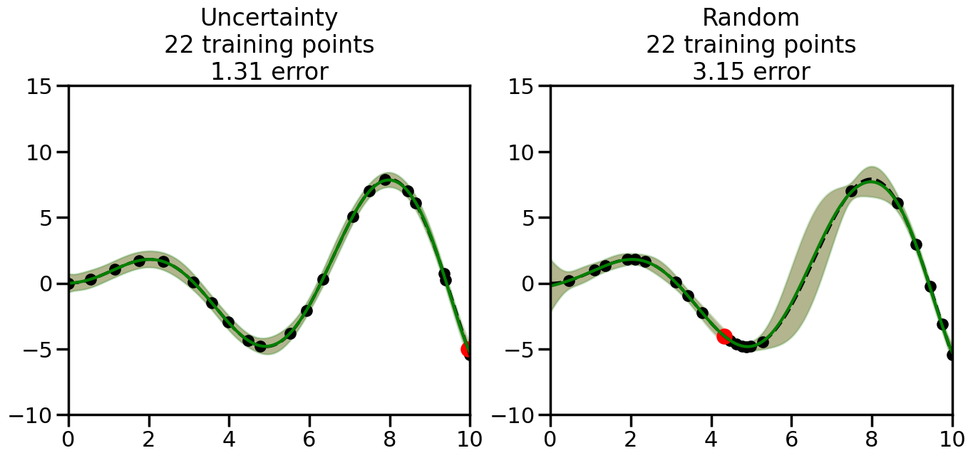
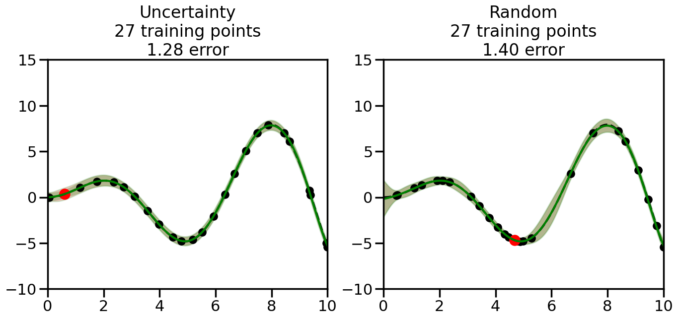
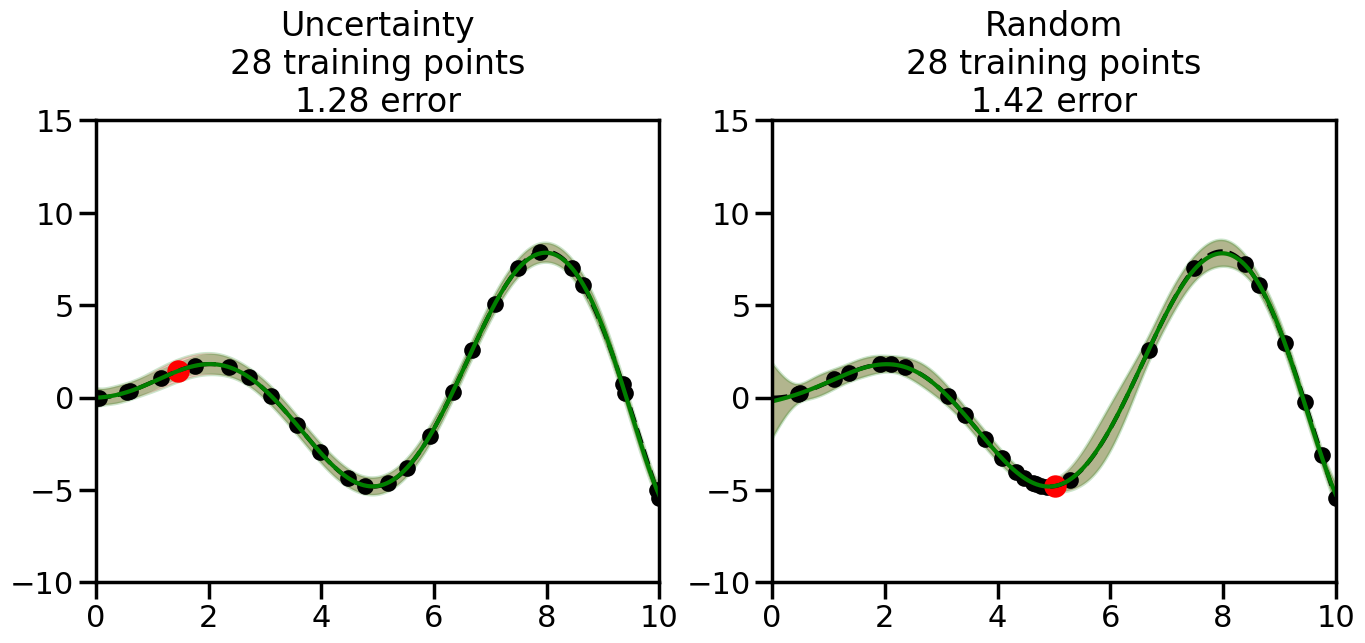
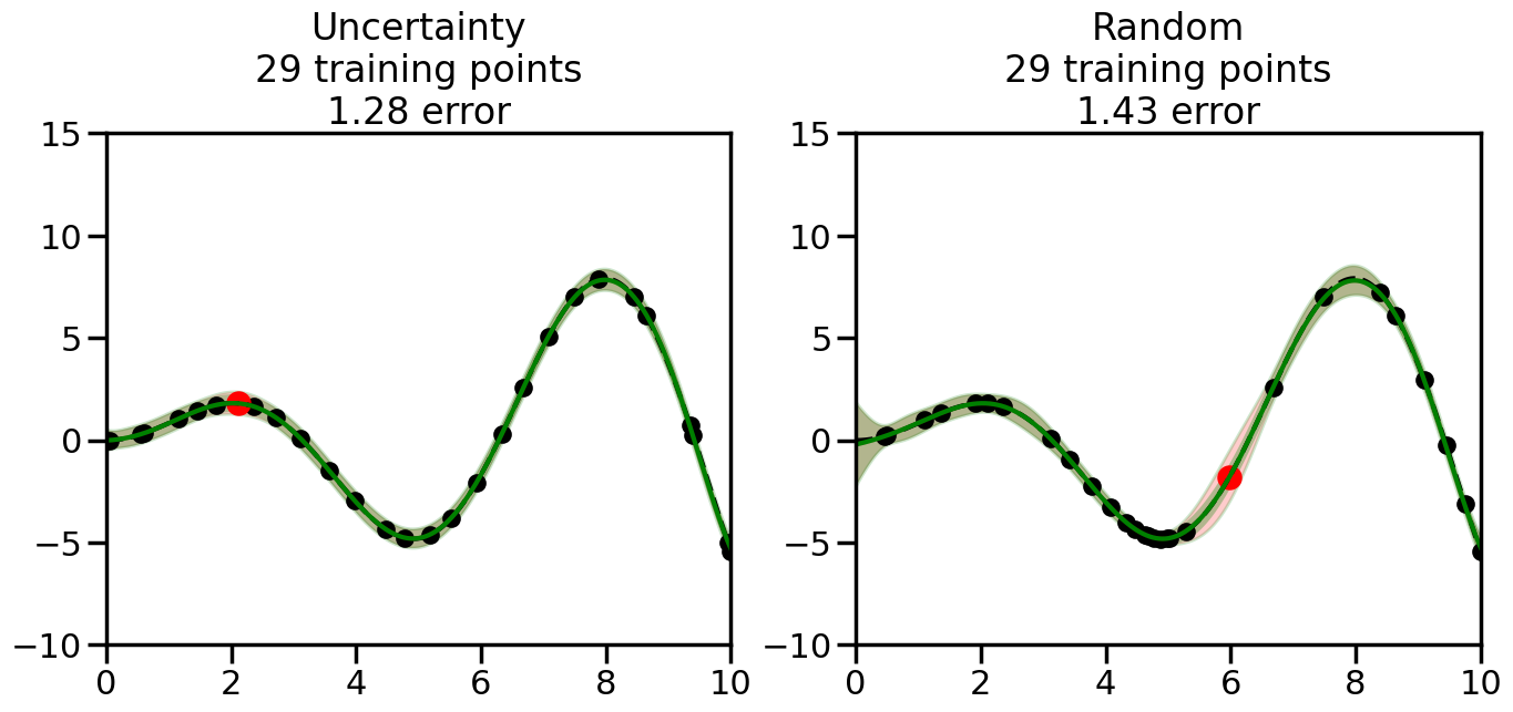
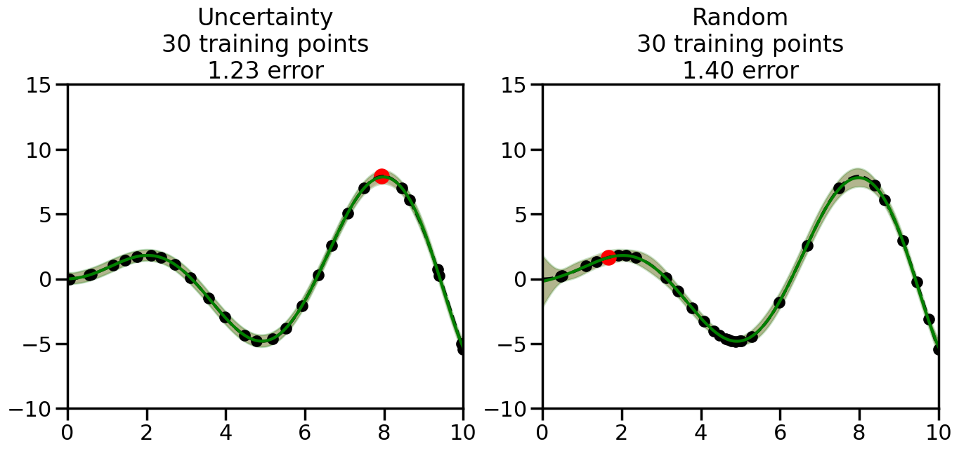
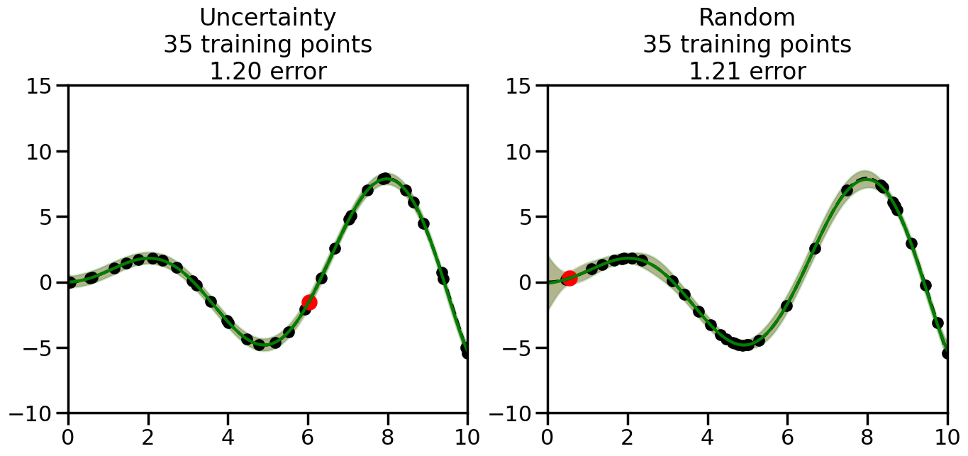
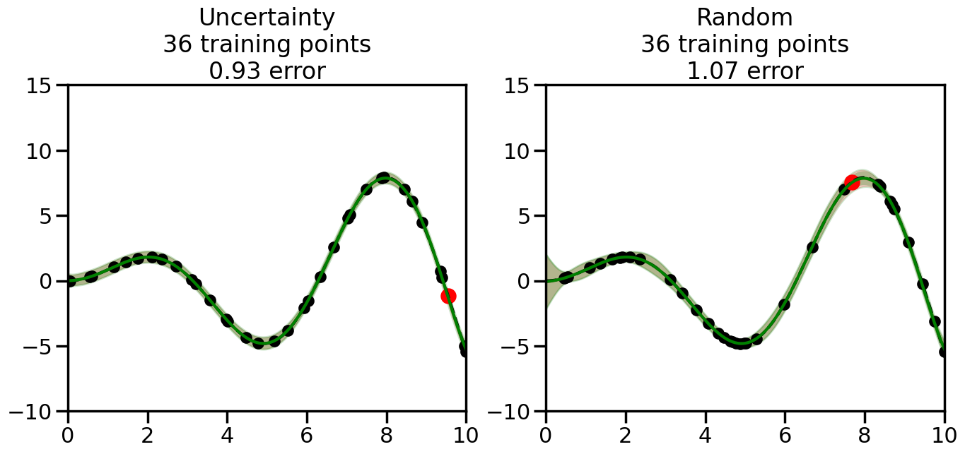
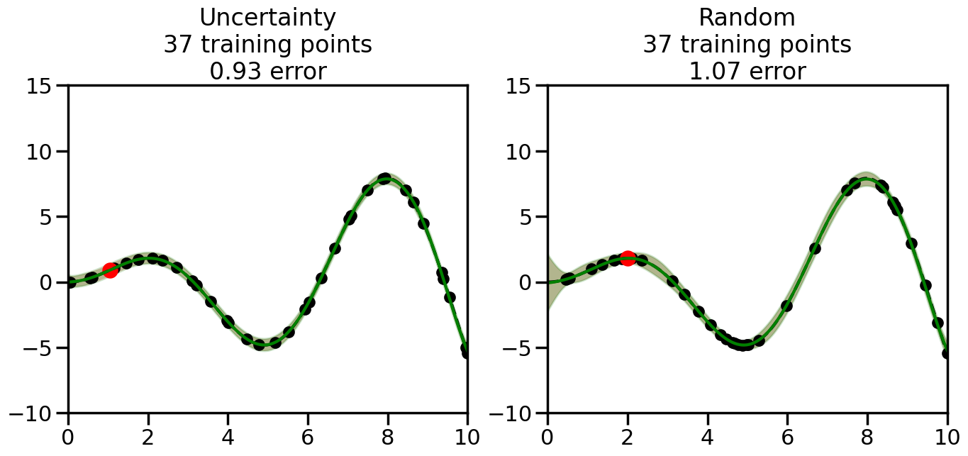
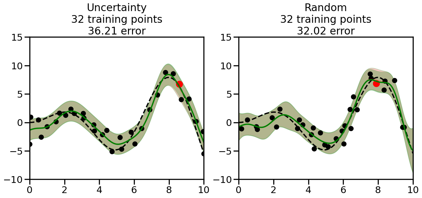
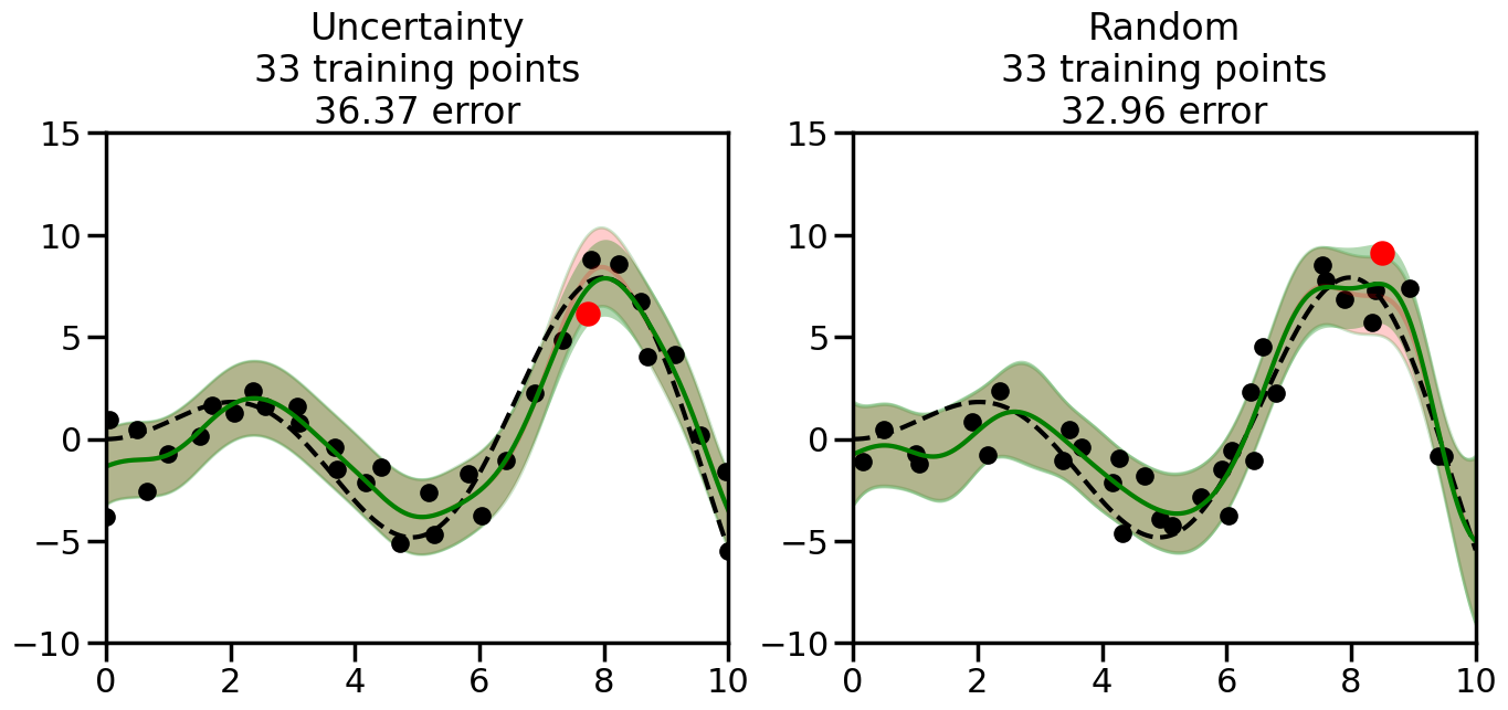
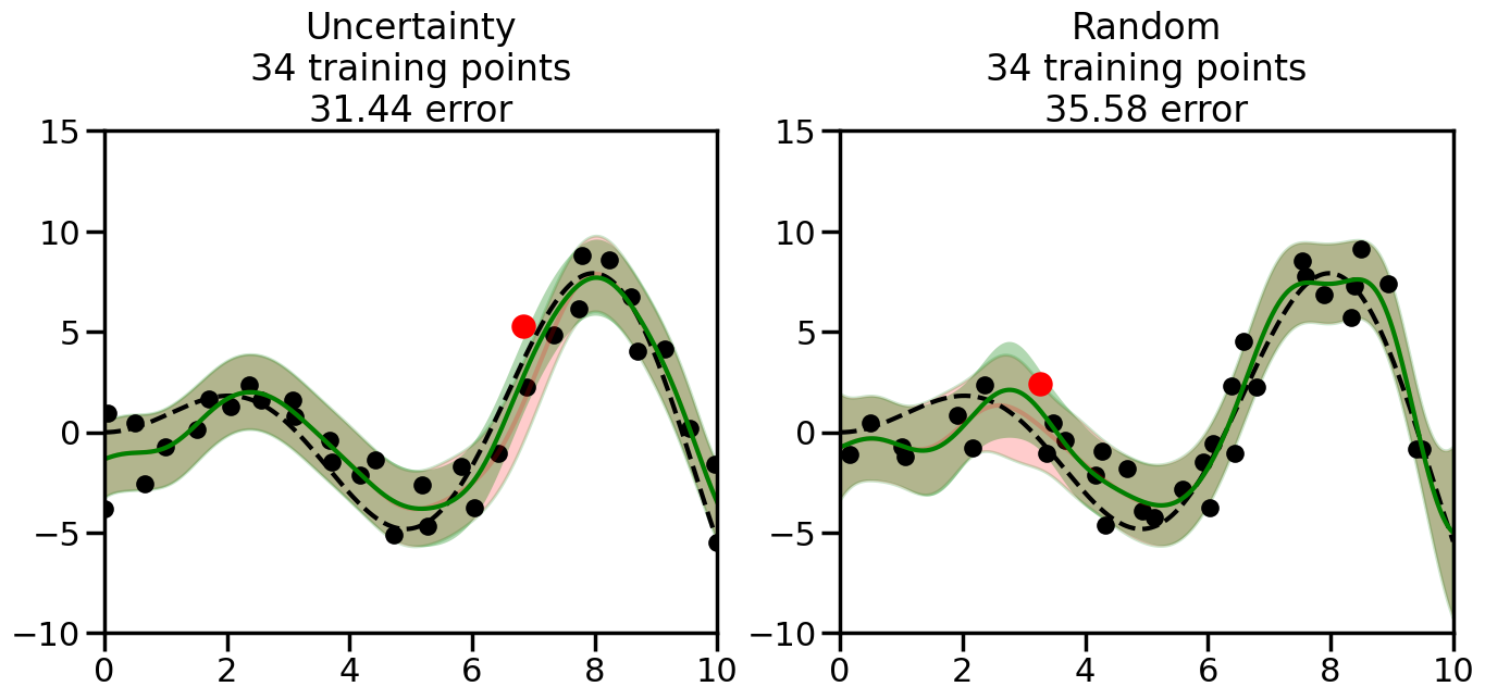
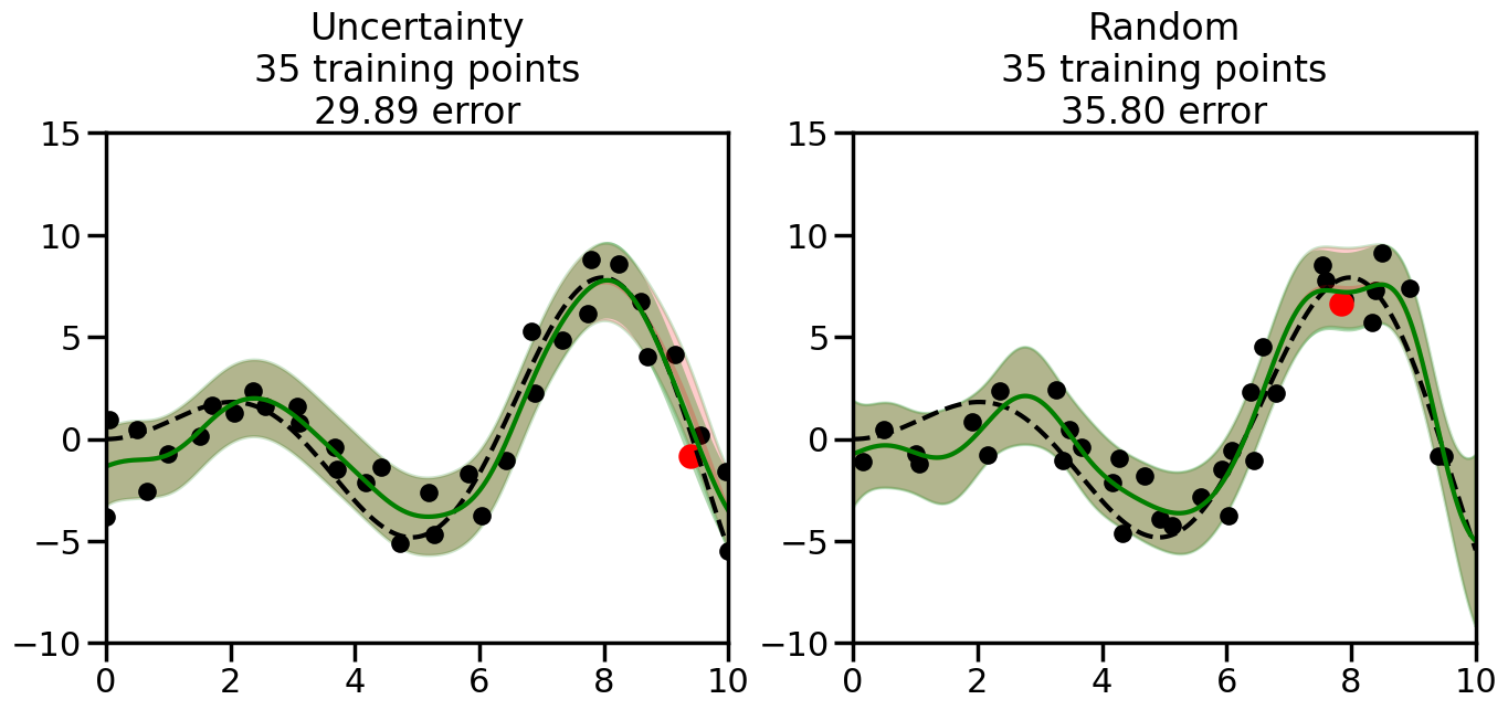
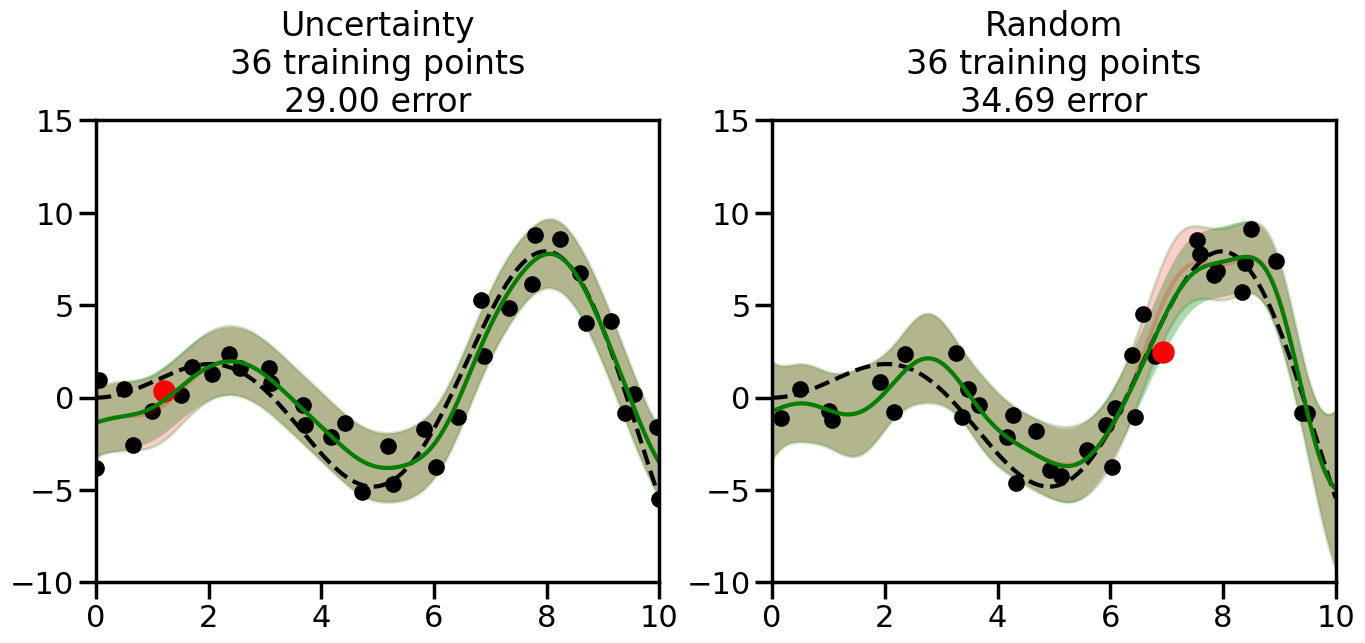
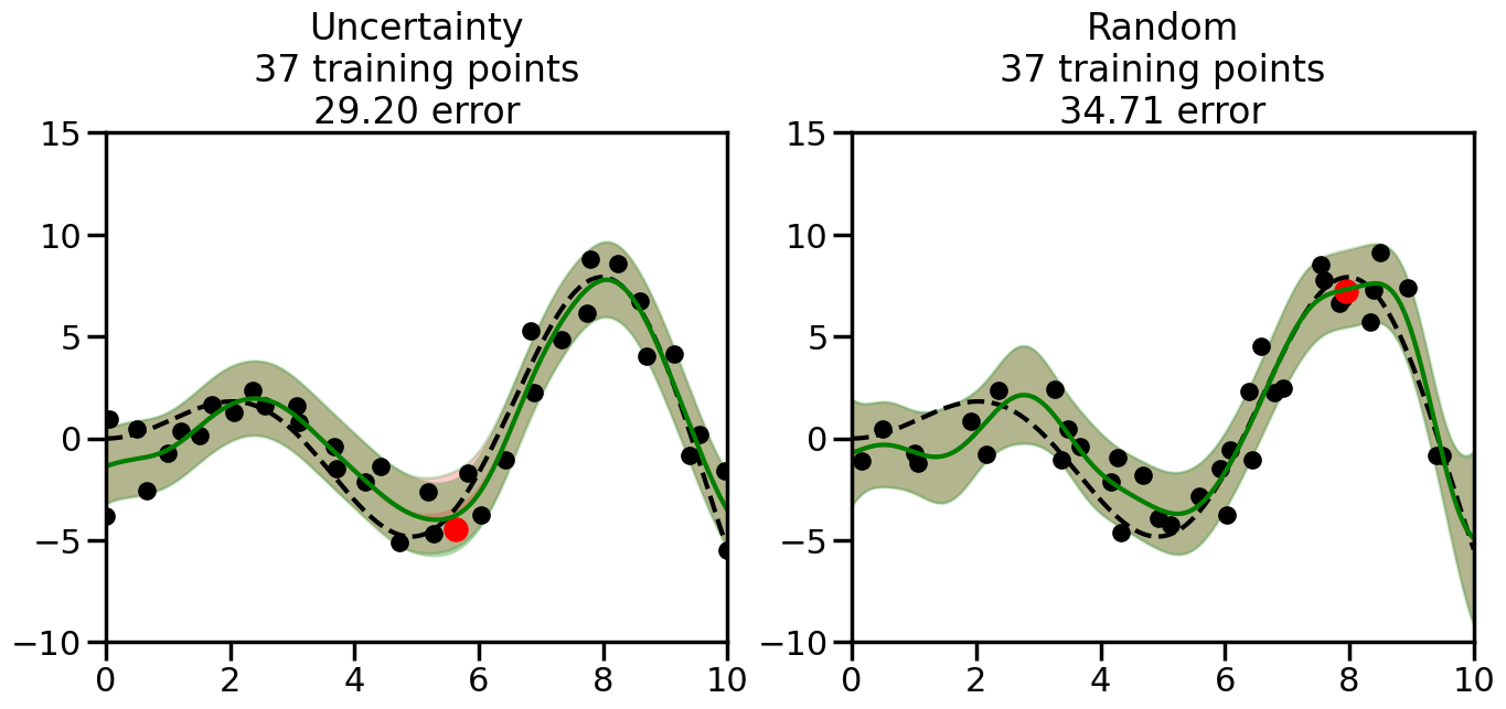
What we will see in the plots below is a red line and shaded region representing the GP model (both mean and variance) before we sampled a new datapoint, and then we will overlay the GP model after we have sampled and added the new datapoint to the training set. The new model will be shown with a green line and shaded region. The selected datapoint will be marked with a large red circle. In Uncertainty Sampling, we should see that the selected datapoint is located where the initial model (red line) has high uncertainty (wide red shaded region). In Random Sampling, the selected datapoint will be chosen randomly from the input space. You can see what happens to the model’s uncertainty as we add the point, as well as the overall Mean Squared Error (MSE) on a held-out test set after each iteration.
# Create the Gaussian Process model# We can start with a basic RBF kernelkernel = RBF(length_scale=1) #+ WhiteKernel(noise_level=0.01)# You can also experiment with adding noise to the kernel to see how this affects the sampling# kernel = RBF(length_scale=1) + WhiteKernel(noise_level=0.01)gp = GaussianProcessRegressor(kernel=kernel, alpha=0.01, optimizer=None, normalize_y=True, random_state=1)def sample_data_points(X, y, gp, num_points=35):"""Compare Uncertainty Sampling vs Random Sampling for Active Learning."""# Now, we are ready to begin learning!# We will have two different models that we'll test out:# 1) Uncertainty Sampling: Pick points where we are most uncertain# 2) Random Sampling: Pick points randomly# train_ind holds the indices of what training samples we'll use train_ind ={'Uncertainty': np.zeros(len(X),dtype=bool),'Random': np.zeros(len(X),dtype=bool) } options = train_ind.keys()# We can now initialize the first few training points. possible_points = np.array(list(range(len(X))))# Possible Initialization options# 1. Start with the same two randomly selected pointsfor ind in np.random.choice(possible_points,2):for o in options: train_ind[o][ind] =True# Or# 2. Start with end-points#for o in options:# train_ind[o][0] = True# train_ind[o][-1] = True# How much data should we collect? num_total_samples =35# Let's store the errors for the models: errors = {'Uncertainty':np.zeros(num_total_samples),'Random':np.zeros(num_total_samples)}# Let's select an increasing number of new points to try:for i inrange(num_total_samples):# As i increases, we increase the number of points plt.figure(figsize=(16,6))for j,o inenumerate(options): # For each sampling option plt.subplot(1,2,j+1) # Create different subplot# Fit the original GP Model (without the new point): gp.fit(X[train_ind[o],:],y[train_ind[o]])# Plot the original model's bounds (just for comparison sake) yp,sigma = gp.predict(x, return_std=True) plt.fill(np.concatenate([x, x[::-1]]), np.concatenate([yp -1.9600* sigma, (yp +1.9600* sigma)[::-1]]),'r', alpha=0.2, ec='g', label='95% confidence interval')# Plot the predicted function plt.plot(x,yp,'r-',alpha=0.2)######## Now do the Active Learning part####### # Here is Uncertainty Sampling:if o =='Uncertainty':# First, we need to predict the MSE (uncertainty) at# each of the non-training points: yp,sigma = gp.predict(X[~train_ind[o],:], return_std=True)# The points that we'll choose from are the points that have the# maximum mean square error in the GP (highest uncertainty) candidates = np.extract(sigma == np.amax(sigma),X[~train_ind[o],:])# Side note:# If you wanted to turn Uncertainty Sampling into Global Bayesian# Optimization instead, then uncomment the below two lines, which implements# Upper Confidence Bound (UCB) sampling:# ucb = yp + 1.96*sigma# candidates = np.extract(ucb == np.amax(ucb),X[~train_ind[o],:])# Choose the next sampling point randomly from the max candidates# (It is unlikely that len(candidates)>1, but you never know) next_point = np.random.choice(candidates.flatten())# Find the training sample index corresponding to the next sample next_ind = np.argwhere(X.flatten() == next_point)# Here is Random Sampling:elif o =='Random':# Just pick the point randomly from the points that we # haven't chosen already (i.e., ~train_ind[o]) next_ind = np.random.choice(possible_points[~train_ind[o]],1)# Add the selected point to the training samples train_ind[o][next_ind] =True######## Done with Active Learning part####### # Fit the GP again, this time with the added training point: gp.fit(X[train_ind[o],:],y[train_ind[o]])# Now plot the updated model so we can see the difference: yp,sigma = gp.predict(x, return_std=True)# Draw the 95% Confidence Interval plt.fill(np.concatenate([x, x[::-1]]), np.concatenate([yp -1.9600* sigma, (yp +1.9600* sigma)[::-1]]),'g', alpha=0.3, ec='None', label='95% confidence interval')# Plot the original function plt.plot(x,f(x),'k--',alpha=1)# Plot the predicted function plt.plot(x,yp,'g-',alpha=1)# Plot the original training points plt.scatter(X[train_ind[o],:],y[train_ind[o]],color='k',s=100)# Highlight the point we just added plt.scatter(X[next_ind,:].flatten(),y[next_ind].flatten(),color='r',s=200) plt.ylim([-10,15]) # Set the y-axis limits plt.xlim([0,10]) # Set the x-axis limits# Label the figure title with the number of total training points# and the total error between the predicted and actual curves n_train = np.count_nonzero(train_ind[o]) error = np.linalg.norm(yp-f(x).flatten()) errors[o][i]=error plt.title("%s\n%d training points\n%.2f error"%(o,n_train,error)) plt.show()return errorserrors = sample_data_points(X, y, gp, num_points=35)
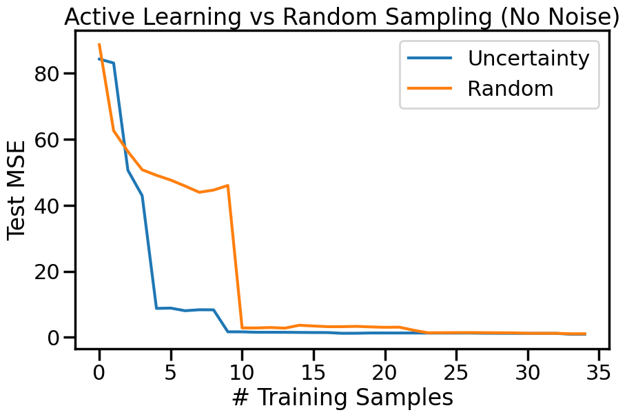
We can also plot the overall Test MSE as a function of the number of labeled datapoints added, to see how quickly each strategy improves the model’s performance:
Code
plt.figure(figsize=(10,6))options = errors.keys()for o in options: # For each sampling option plt.plot(errors[o],label=o)plt.legend()plt.xlabel("# Training Samples")plt.ylabel("Test MSE")plt.title("Active Learning vs Random Sampling (No Noise)")plt.show()
23.4.1 Uncertainty Sampling under Noise
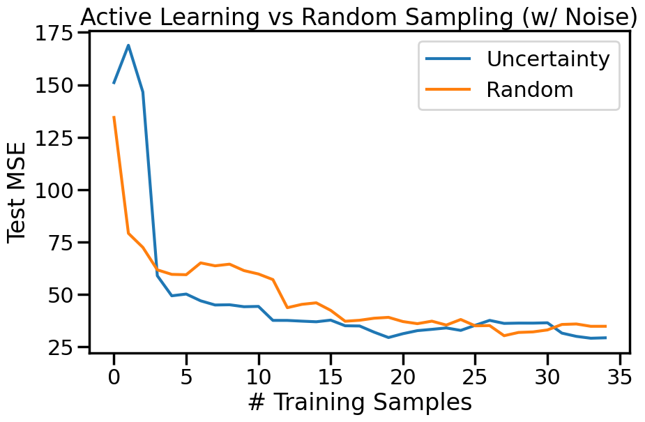
While the above example shows the effectiveness of uncertainty sampling in a noise-free scenario, real-world data is often noisy. To simulate this, we can add Gaussian noise to our observations. This will help us understand how uncertainty sampling performs when the data is not perfectly clean. Intuitively, we expect that uncertainty sampling will still be effective, but the presence of noise may lead to selecting points that are not as informative as in the noise-free case, and that as the noise increases the benefits we accrue from Active Learning may diminish. We can modify the previous example code to include Gaussian noise in the observations and observe how the model’s performance changes with uncertainty sampling compared to random sampling.
Code
# ------- Try changing the below to include the GP and noise -------noise_factor =1.5# e.g. between 0 and 5RBF_length_scale =0.8# e.g., between 0.1 and 5# --------------------------------------# np.random.seed(1)# def f(x):# """The function to predict."""# return x * np.sin(x)# #return 5 * np.sinc(x)# #return x# #----------------------------------------------------------------------# # First the noiseless case# X = np.atleast_2d(np.linspace(0, 10, 40)).T# Observationsy = f(X).ravel() # Noiseless observations# Add some noise#dy = 0.5 + 1.0 * np.random.random(y.shape)#noise = np.random.normal(0, noise_factor*dy)noise = np.random.normal(0, noise_factor, size=y.shape)y_noisy = y + noise# Create the Gaussian Process modelkernel_noisy = RBF(length_scale=RBF_length_scale, length_scale_bounds=(0.5, 1.5)) +\ WhiteKernel(noise_level=0.05,noise_level_bounds=(0.01, 0.2))gp_noisy = GaussianProcessRegressor(kernel=kernel_noisy, n_restarts_optimizer =10, optimizer=None, # 'fmin_l_bfgs_b' or None normalize_y=True, random_state=1)errors_noisy = sample_data_points(X, y_noisy, gp_noisy, num_points=35)
Code
plt.figure(figsize=(10,6))for o in options: # For each sampling option plt.plot(errors_noisy[o],label=o)plt.legend()plt.xlabel("# Training Samples")plt.ylabel("Test MSE")plt.title("Active Learning vs Random Sampling (w/ Noise)")plt.show()
TipExperiment: Comparison of Uncertainty and Random Sampling
Go to the above cells and re-run the model with different levels of noise and different RBF length scales. Observe how the performance of Uncertainty Sampling compares to Random Sampling in each case. Consider the following questions:
What happens to Uncertainty Sampling compared to Random Sampling as we increase the noise in the data?
What happens to Uncertainty Sampling compared to Random as we decrease the RBF length scale (i.e., allow more high frequency function behavior)?
23.5 Uncertainty Sampling of Classification Boundaries
We can apply the same ideas behind uncertainty sampling to classification problems as well. In this case, instead of using a Gaussian Process regression model, we can use a Gaussian Process classification model (or any other probabilistic classification model that provides uncertainty estimates). The key idea remains the same: we want to select data points for which the model is most uncertain about the predicted class label.
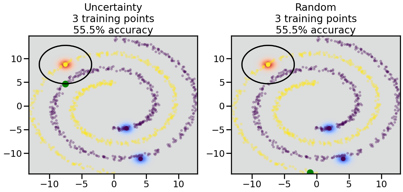
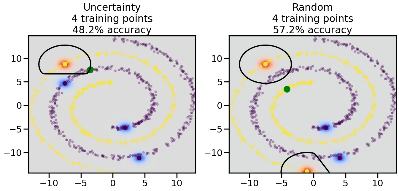
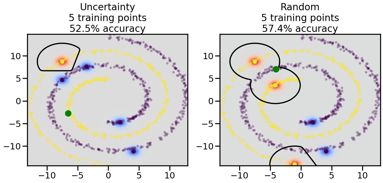
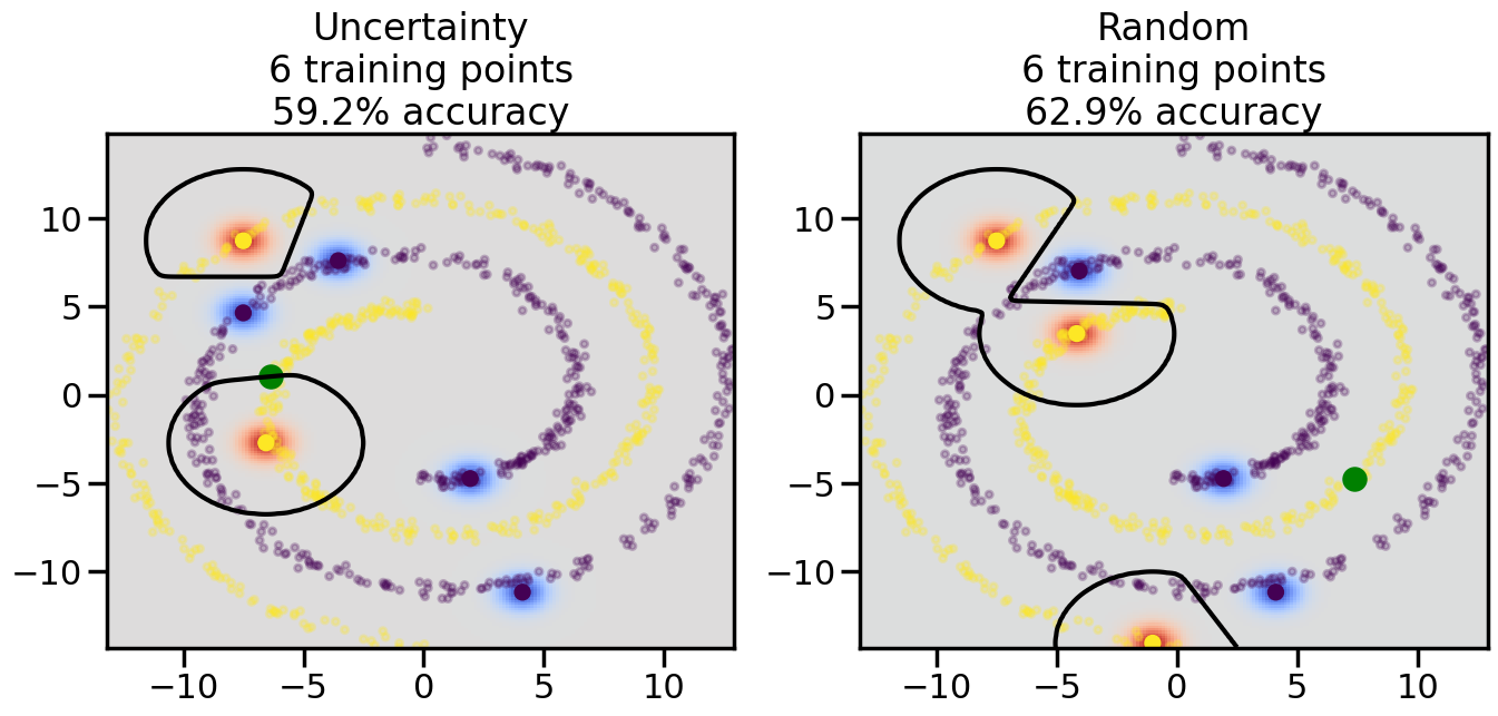
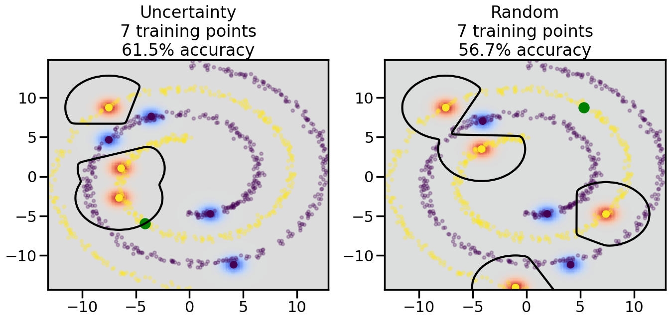
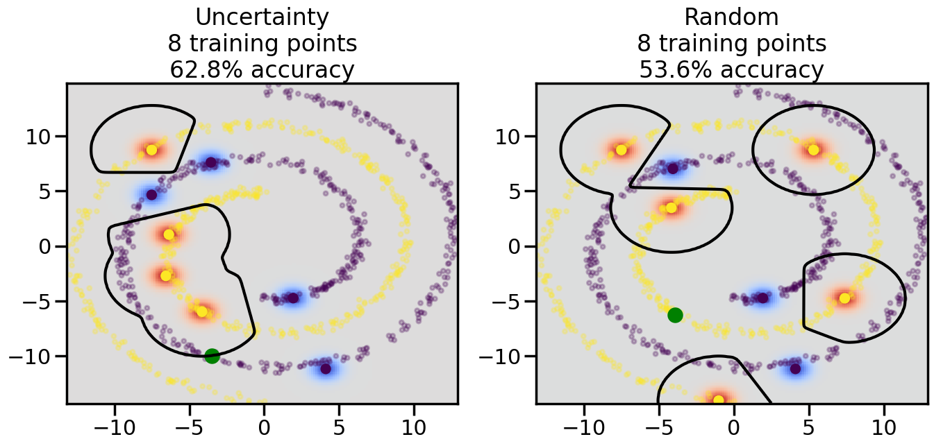
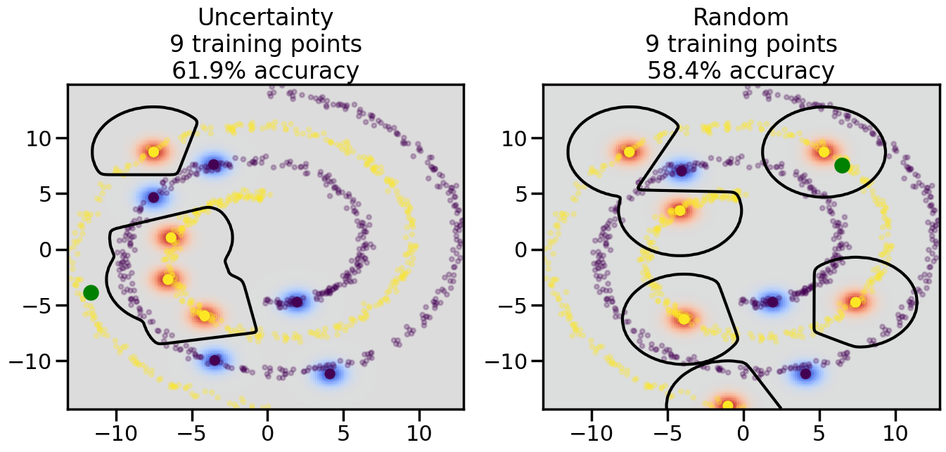
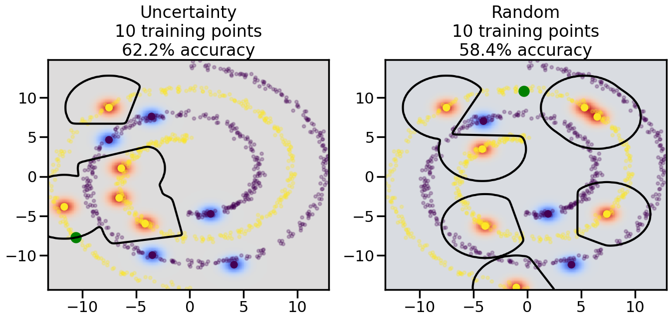
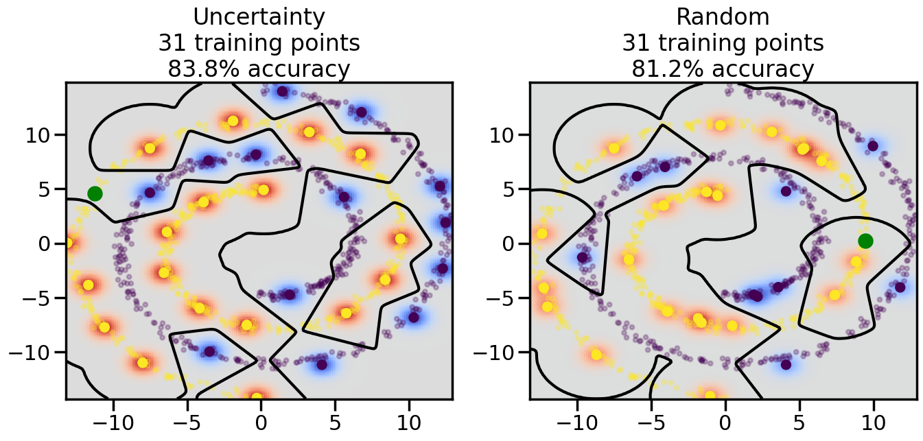
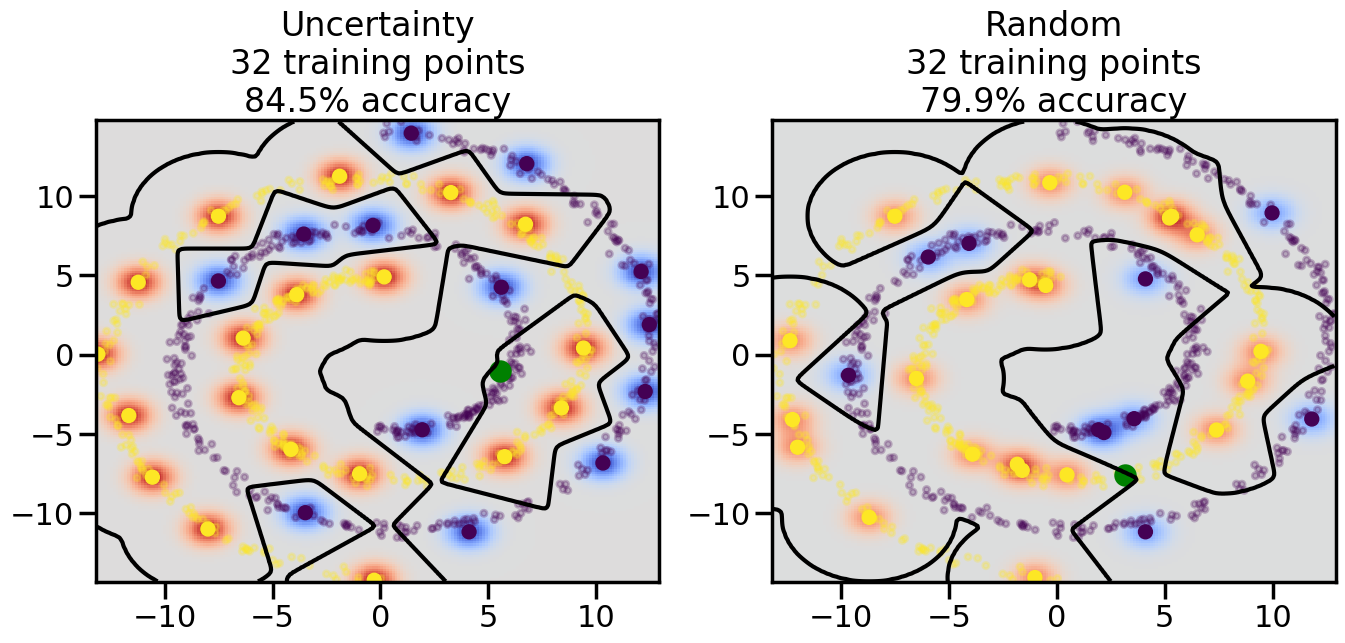
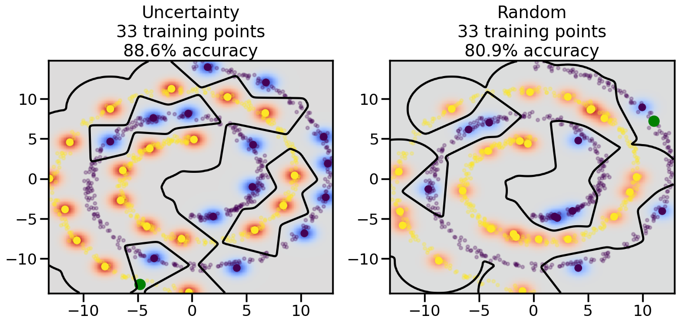
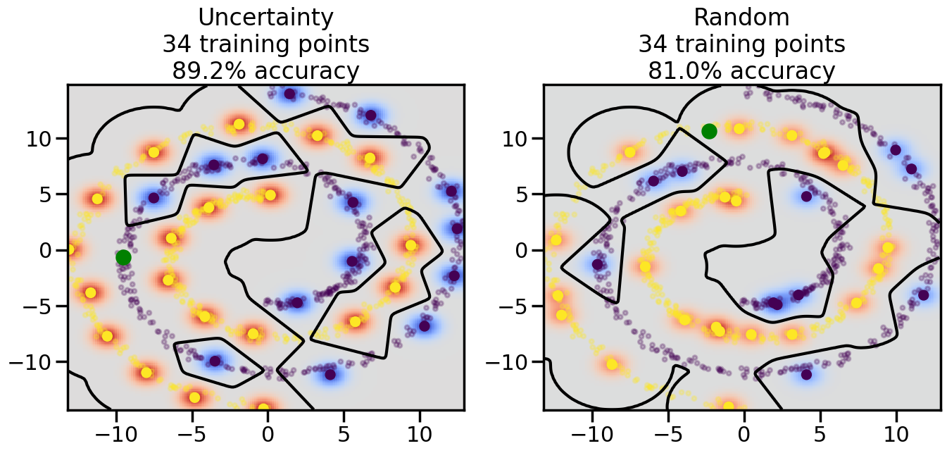
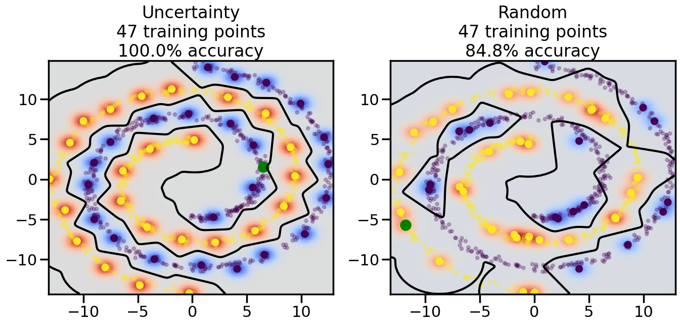
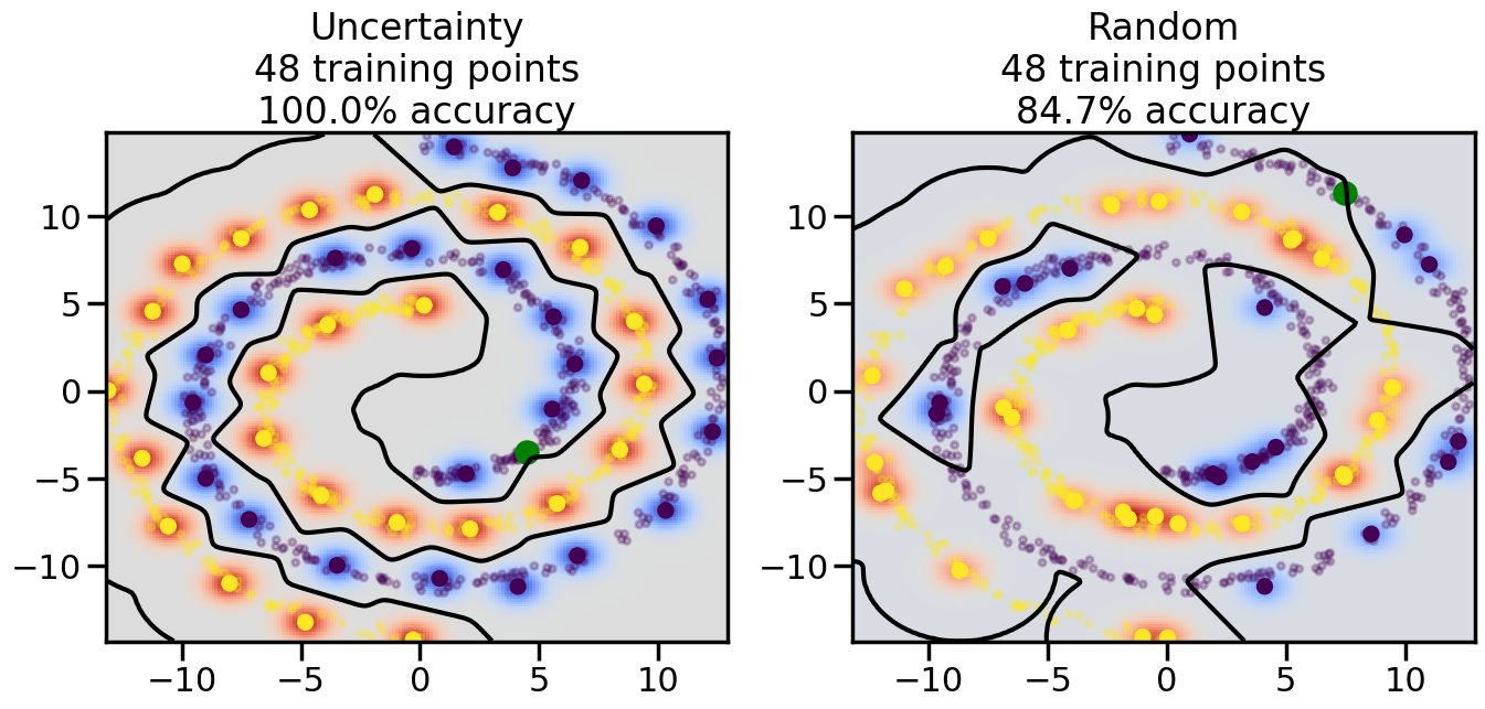
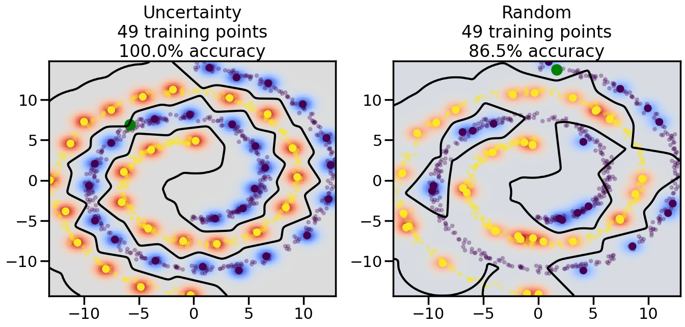
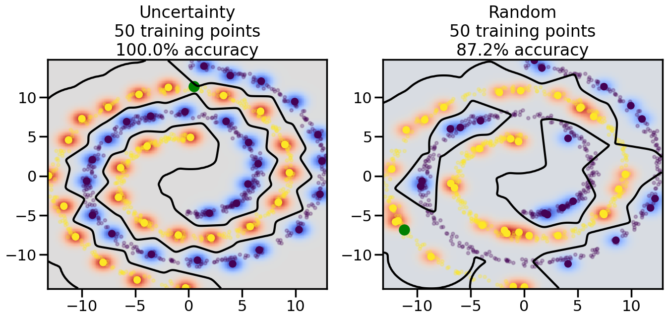
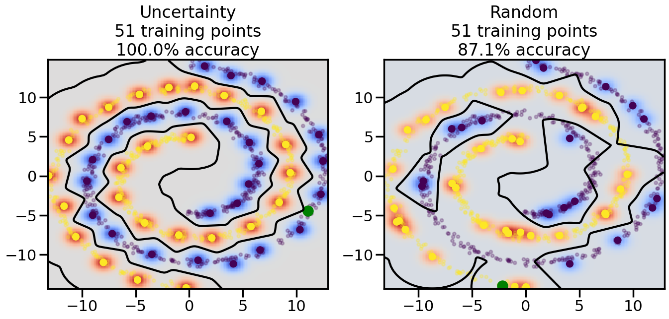
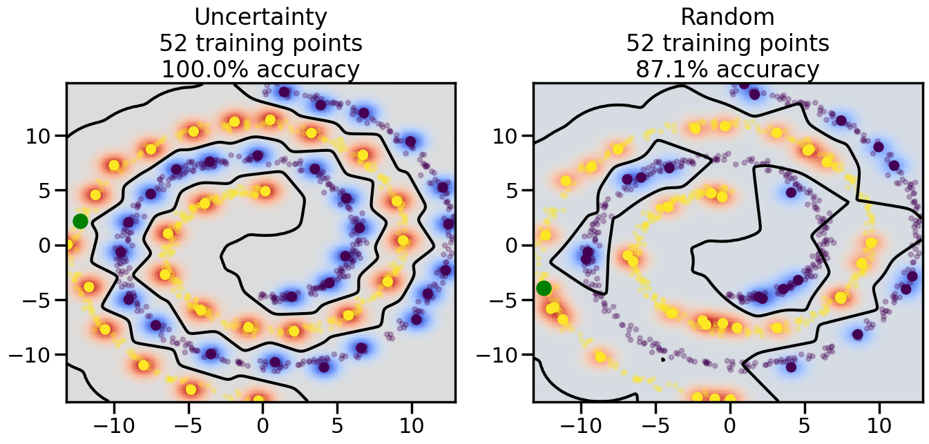
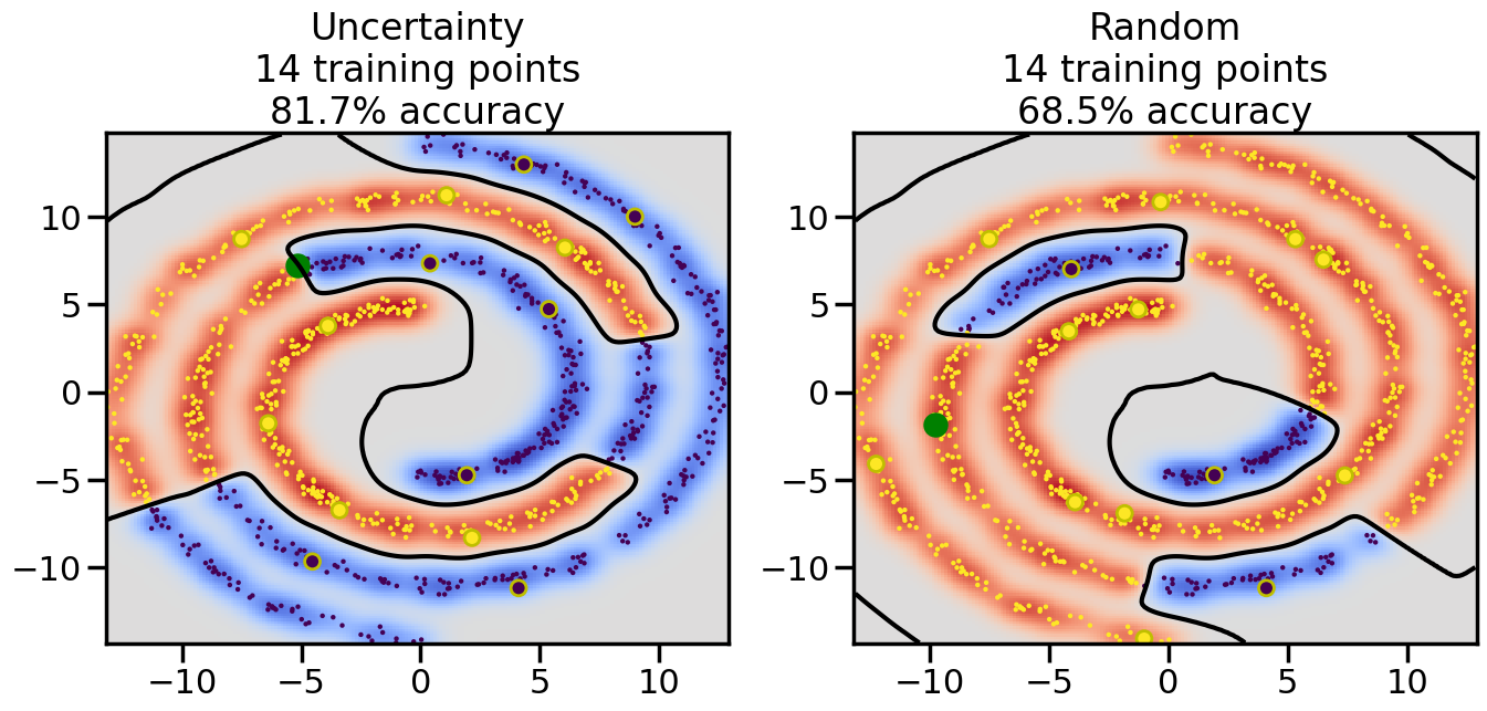
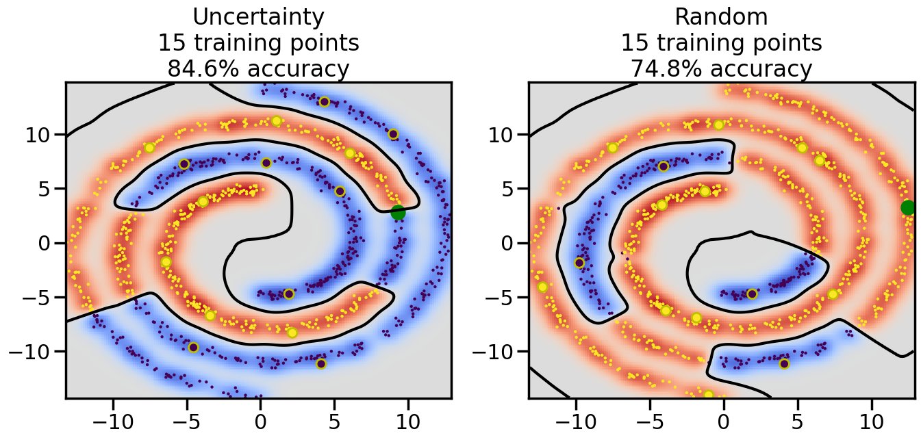
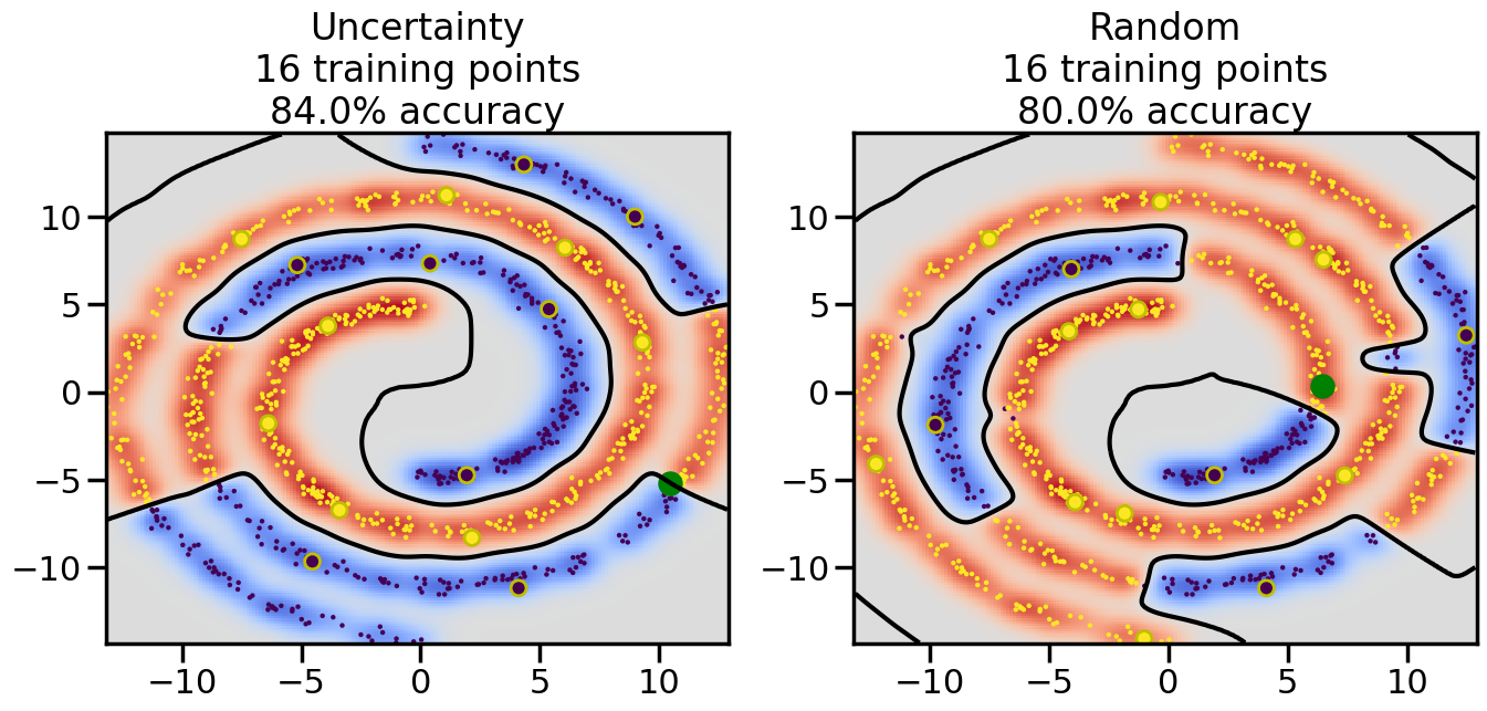
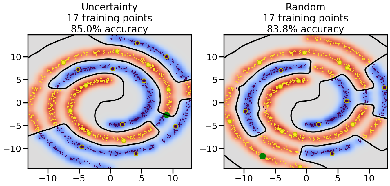
Compare the number of training samples and the Classification Accuracy across the Uncertainty Sampling and Random conditions. You can also try changing the noise parameter for the Moon’s dataset and looking at how that affects things.
Pay special attention to which points the algorithms pick out for training, and how the resulting training data look different after 50-ish iterations.
Code
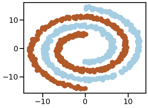
from sklearn.datasets import make_swiss_roll# Make a double roll datasetdef roll_it(n_samples=1000, noise=0.0): X1 = make_swiss_roll(n_samples=int(n_samples/2),noise=noise)[0][:,[0,2]] X2 = make_swiss_roll(n_samples=int(n_samples/2),noise=noise)[0][:,[0,2]] X = np.vstack([X1,-X2]) y = np.hstack([[0]*len(X1),[1]*len(X2)])return X,y
# 2-D Non-Linear Classification# Moons datasetfrom sklearn.datasets import make_moons,make_circlesnp.random.seed(3) # So we all see the same thingn_samples =1000# Number of data samples# ------------------- Try Uncommenting the Below --------------# Dataset 1# Low NoiseX, y = make_moons(n_samples=n_samples, noise=0.1)# Higher Noise# X, y = make_moons(n_samples=n_samples, noise=0.25)# Dataset 2X,y = make_circles(n_samples = n_samples, factor=0.7, noise =.05)# Dataset 3X,y = roll_it(n_samples,0.05*5)# Dataset 4# X, y = make_moons(n_samples=n_samples, noise=0.1)# Xt=np.random.multivariate_normal([-0.7,1.5],np.diag([0.01,0.01]),size=20)# X = np.r_[X,Xt]# y = np.r_[y,np.ones(len(Xt))]# ---------------------------------------------------------------plt.figure()plt.scatter(X[:, 0], X[:, 1], c=y, cmap=plt.cm.Paired)plt.axis('tight')plt.show()
Code
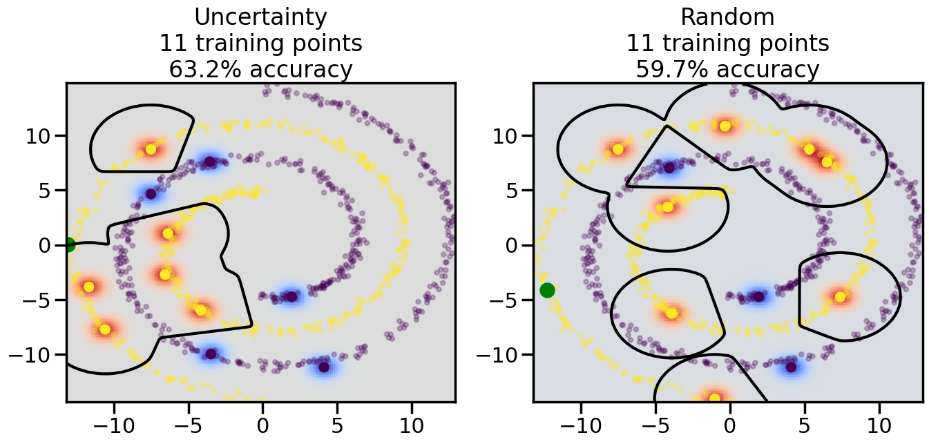
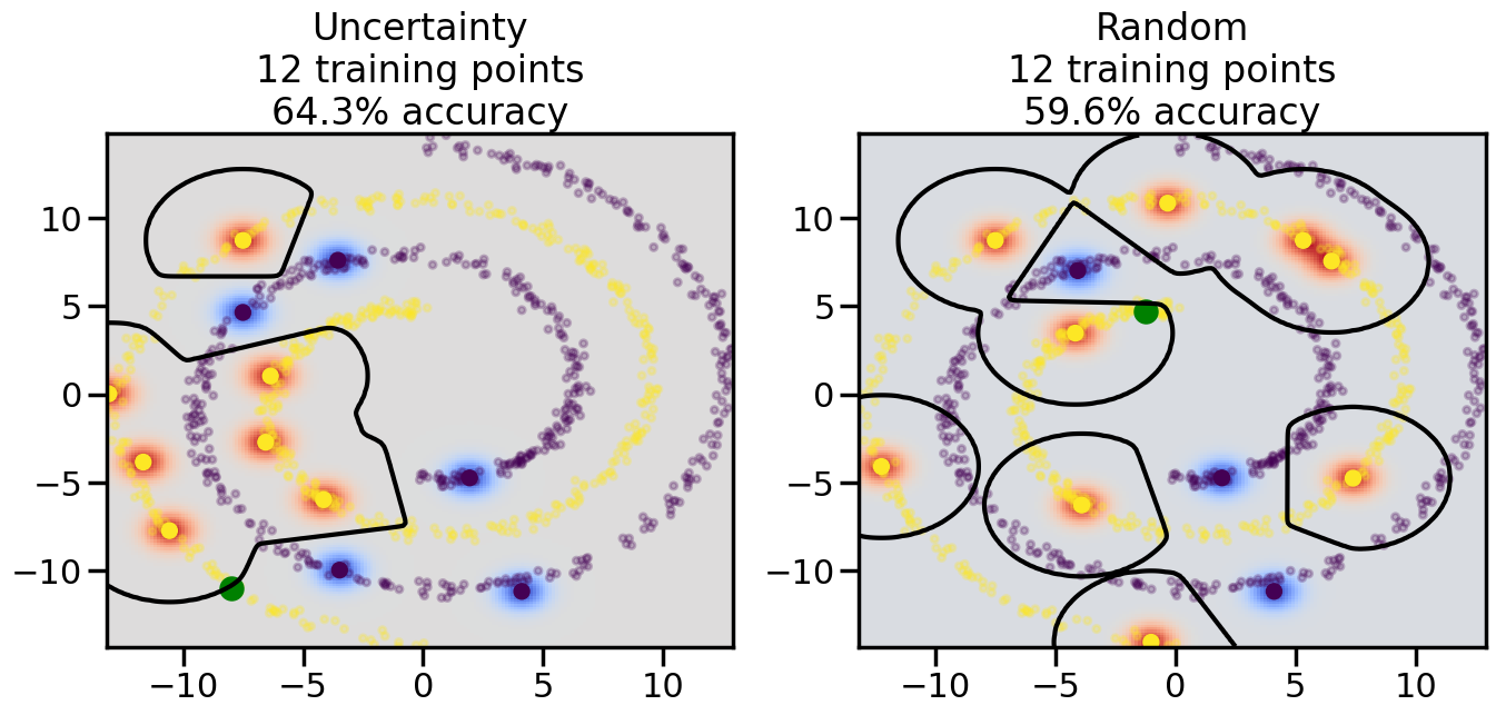
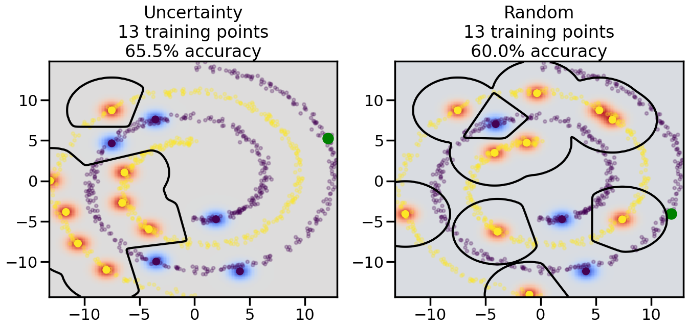
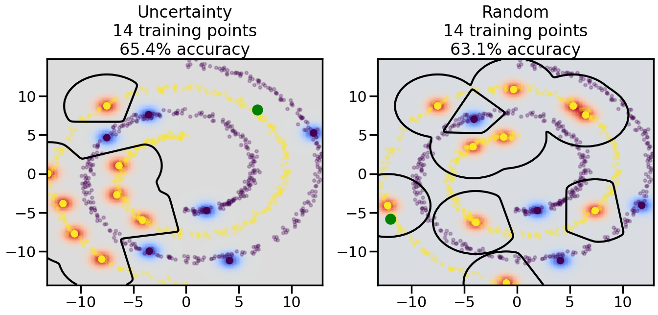
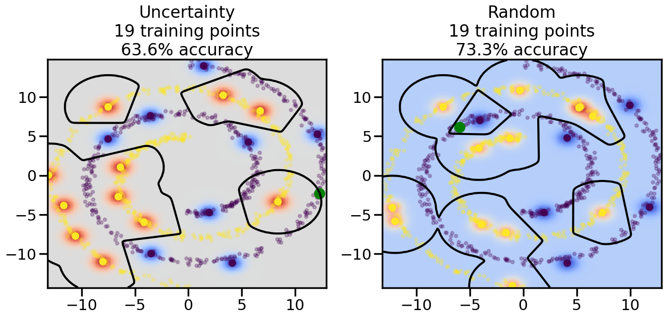
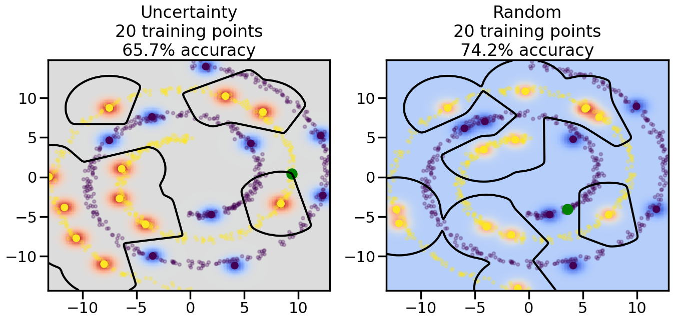
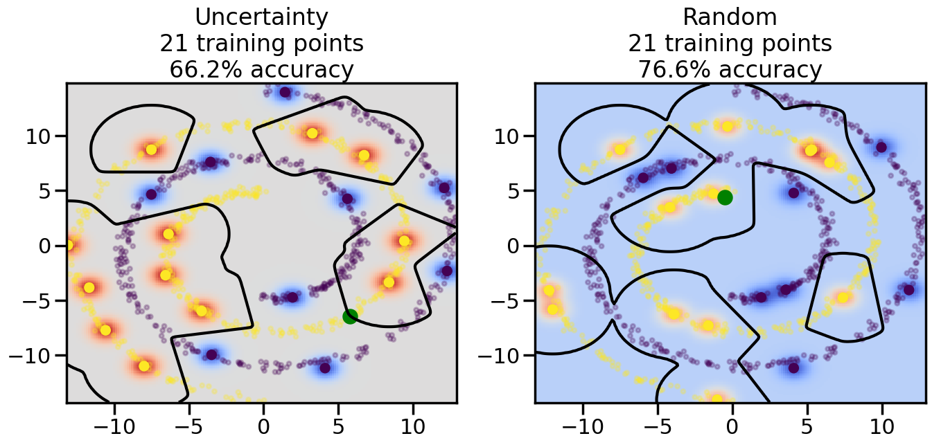
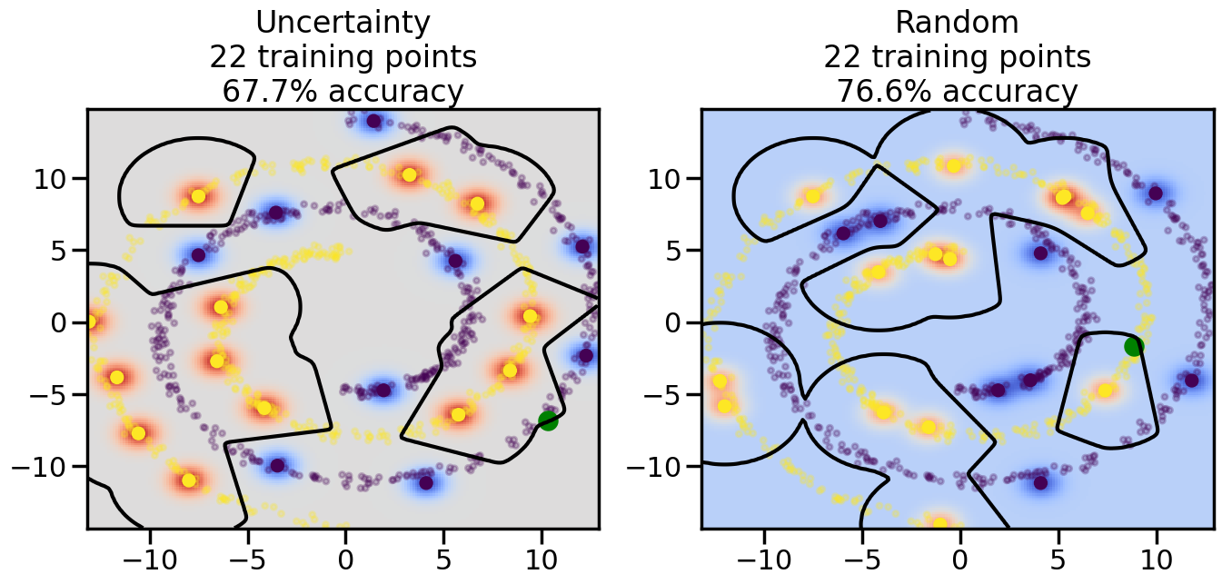
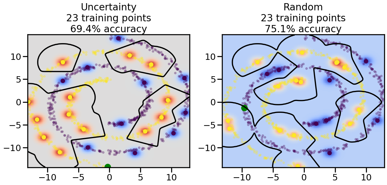
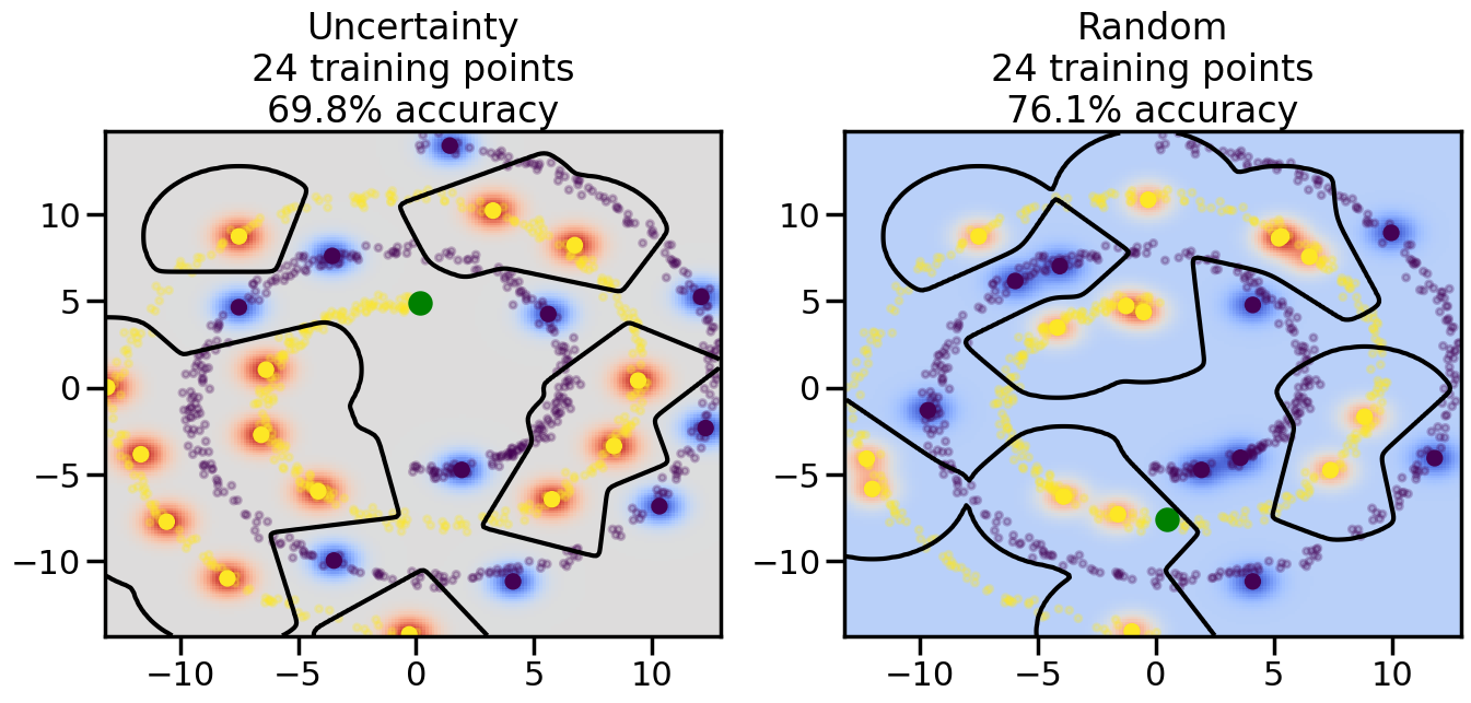
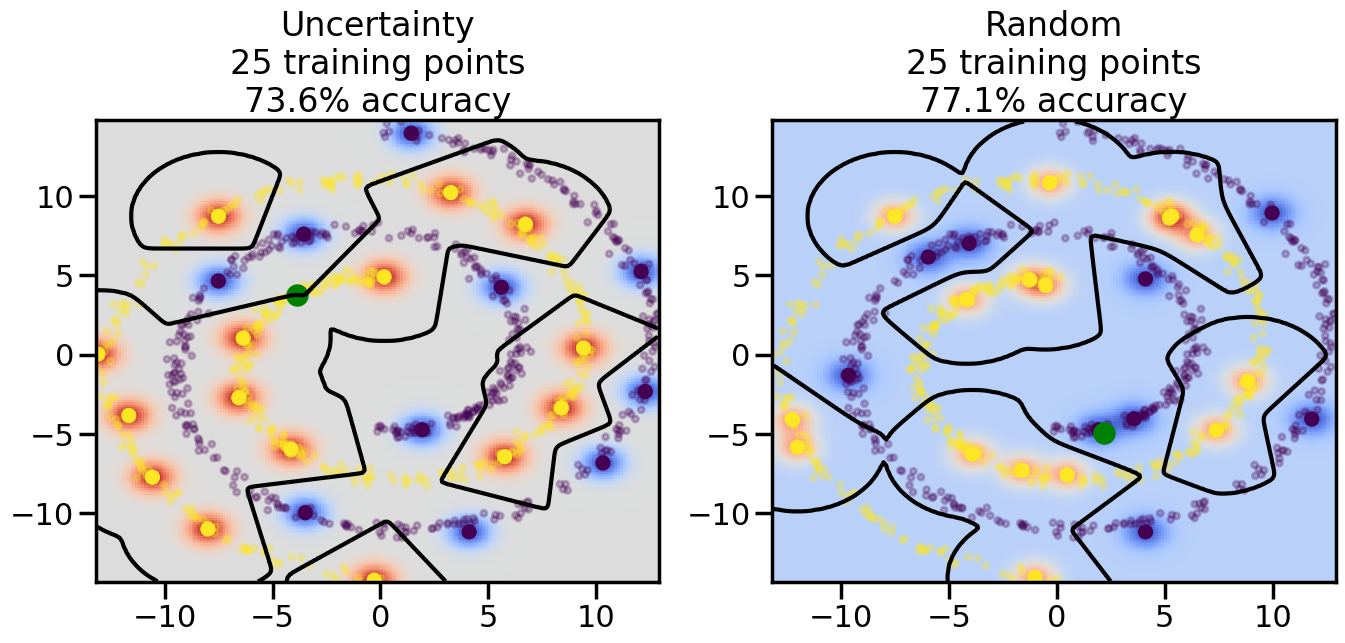
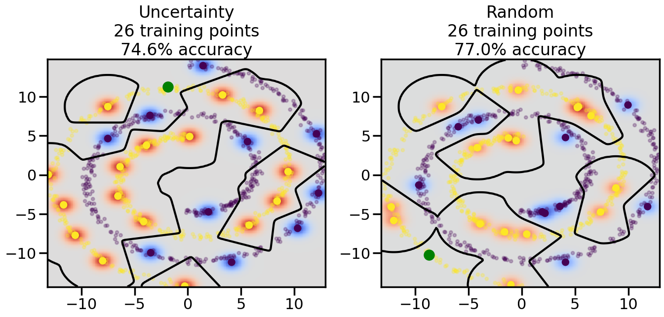
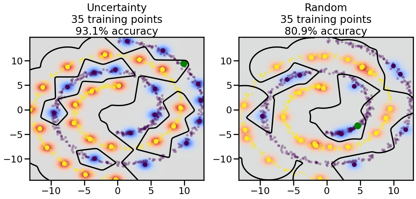
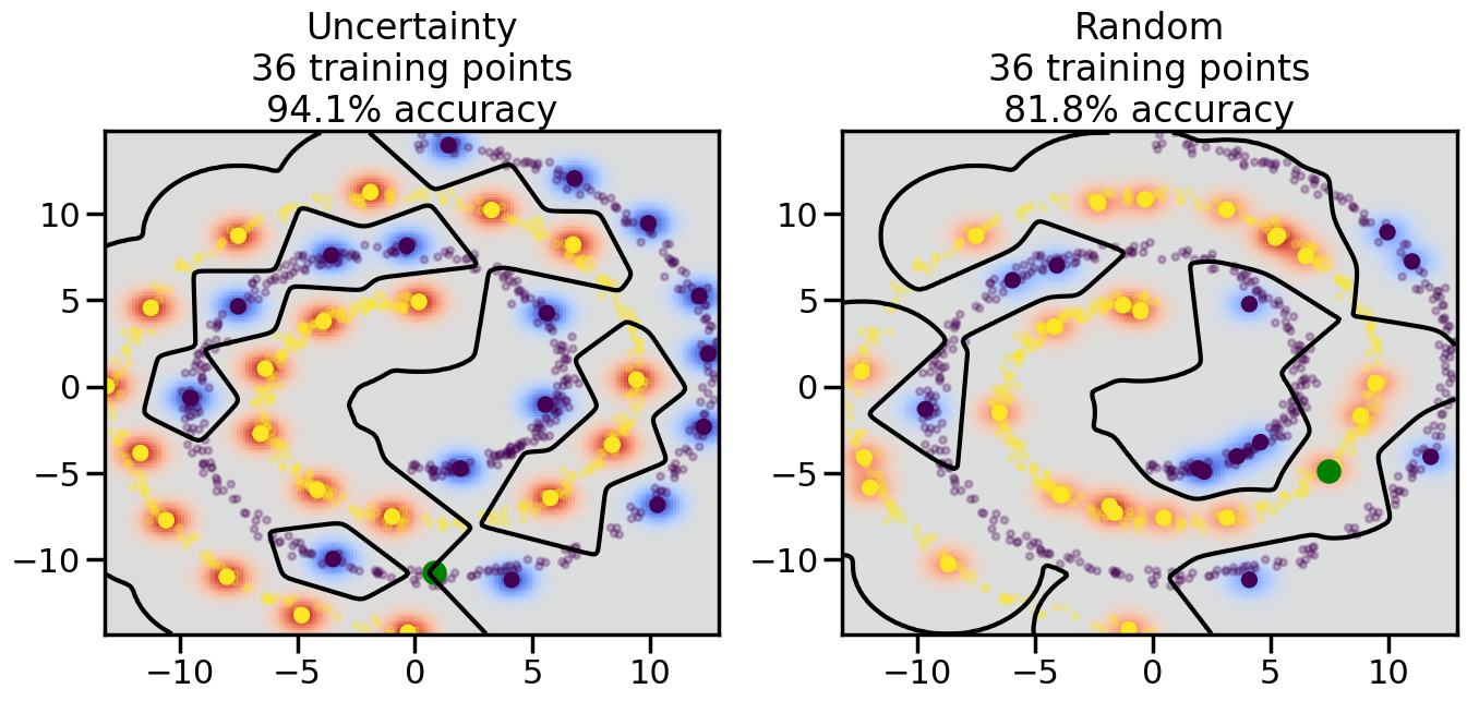
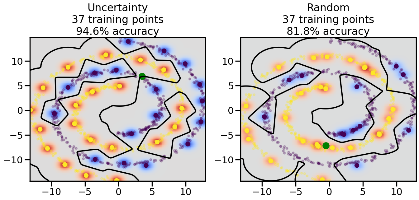
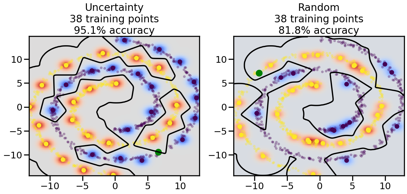
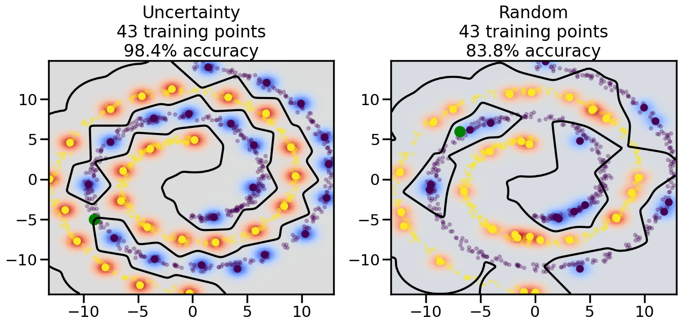
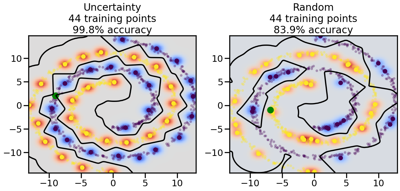
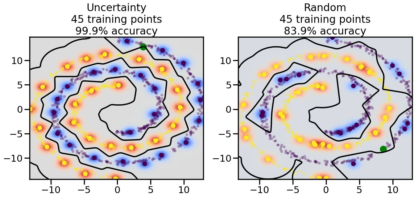
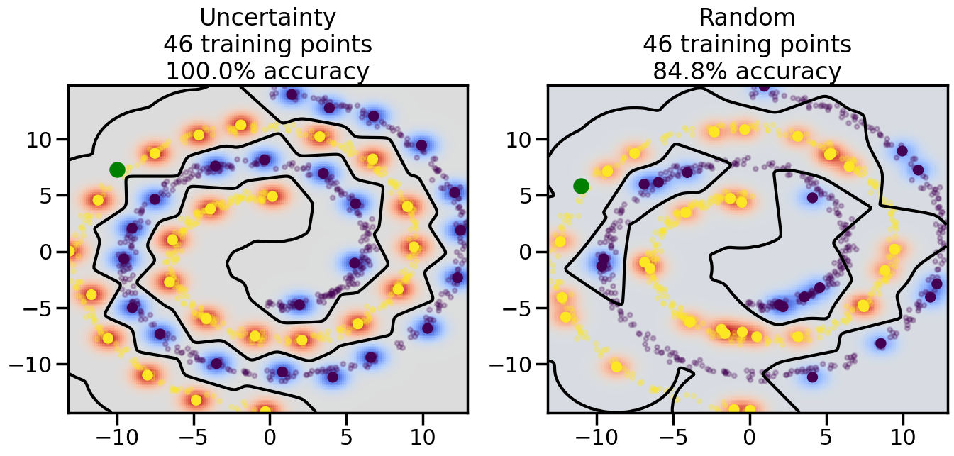
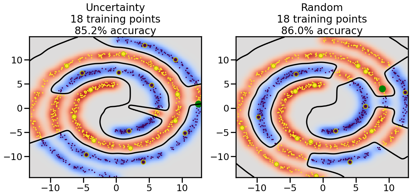
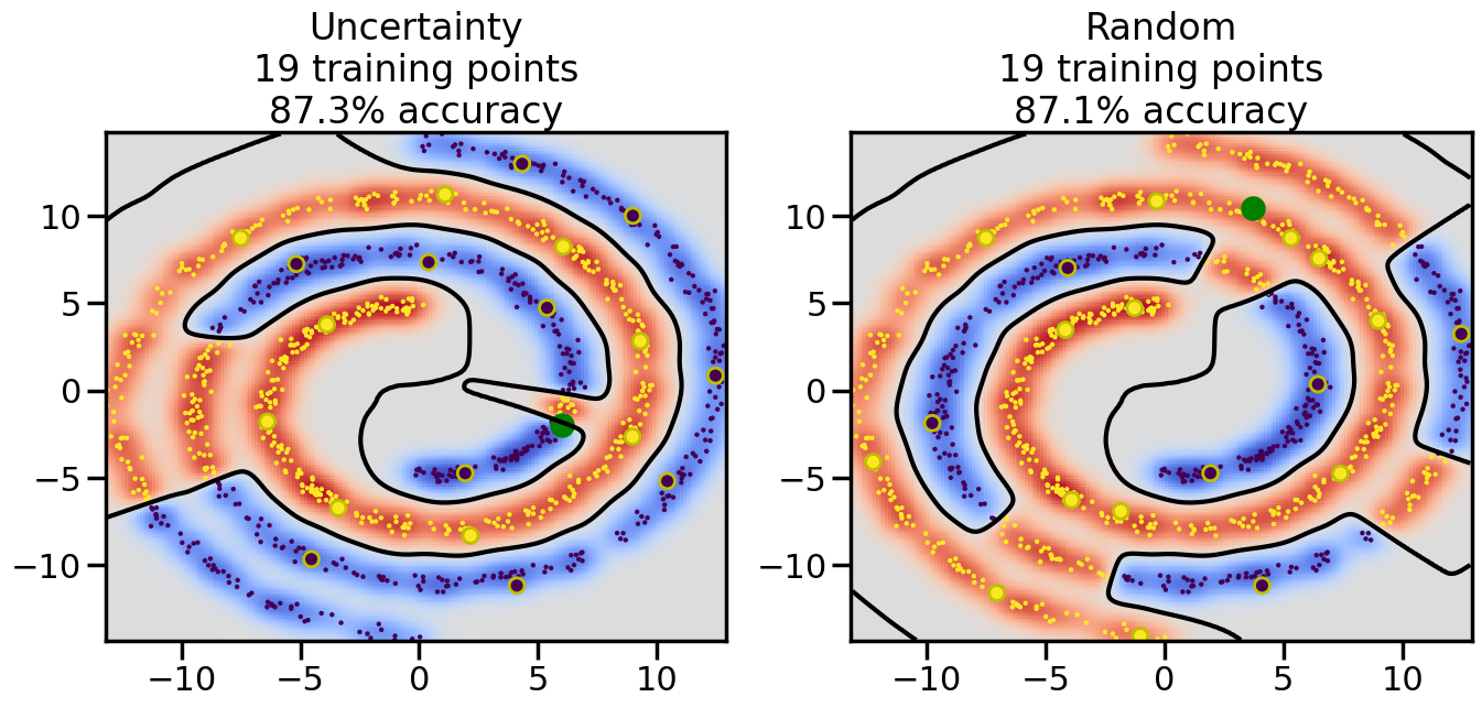
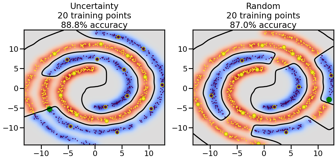
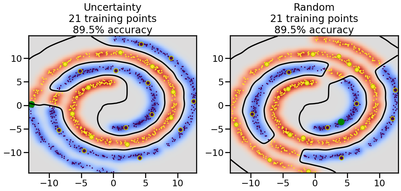
# ------- Try changing the below -------gamma =0.7# e.g. between 0.1 and 5# --------------------------------------#np.random.seed(3)# Now, ready to begin learning:train_ind ={'Uncertainty': np.zeros(len(X),dtype=bool),'Random':np.zeros(len(X),dtype=bool)}options = train_ind.keys()possible_points = np.array(list(range(len(X))))# Initialization options# 1. Select different points randomlyfor i inrange(3): ind = np.random.choice(possible_points[y==i%2])for o in options: train_ind[o][ind] =True# Trying different classifiers#clf = svm.SVC(kernel='rbf',gamma=gamma)clf = GaussianProcessClassifier(1.0* RBF(length_scale=gamma),optimizer=None)# How much data should we collect?num_total_samples =50# Let's store the errors for the models:errors = {'Uncertainty':np.zeros(num_total_samples),'Random':np.zeros(num_total_samples)}for i inrange(num_total_samples):# As i increases, we increase the number of points plt.figure(figsize=(16,6))for j,o inenumerate(options): plt.subplot(1,2,j+1) # Get data on original model (before we select next point) n_train = np.count_nonzero(train_ind[o]) clf.fit(X[train_ind[o],:],y[train_ind[o]]) accuracy = clf.score(X[~train_ind[o],:],y[~train_ind[o]])# Plot the decision function x_min = X[:, 0].min() x_max = X[:, 0].max() y_min = X[:, 1].min() y_max = X[:, 1].max() XX, YY = np.mgrid[x_min:x_max:200j, y_min:y_max:200j]#Z = clf.decision_function(np.c_[XX.ravel(), YY.ravel()]) Z = clf.predict_proba(np.c_[XX.ravel(), YY.ravel()])[:,1] -0.5# Put the result into a color plot Z = Z.reshape(XX.shape) plt.pcolormesh(XX, YY, Z, cmap=plt.get_cmap('coolwarm'),shading='auto') plt.contour(XX, YY, Z, colors=['k', 'k', 'k'], linestyles=['--', '-', '--'], levels=[-.5, 0, .5])# Plot the training points plt.scatter(X[:,0],X[:,1],c=y,s=20,alpha=0.25) plt.scatter(X[train_ind[o],0],X[train_ind[o],1], c=y[train_ind[o]],s=100,lw=1)#clf.fit(X[train_ind[o],:],y[train_ind[o]])#yp,MSE = clf.predict(X[~train_ind[o],:])# Calculate distance to decision boundary# (We're less certain at the boundary)#dists = clf.decision_function(X[~train_ind[o],:]) dists = clf.predict_proba(X[~train_ind[o],:])[:,1] -0.5 dists = np.abs(dists) # Want absolute distance from boundaryif o =='Uncertainty':# Basic Uncertainty sampling# Compute closest points and then pick randomly among# the closet points closest_points = np.argwhere(dists == np.amin(dists)).ravel() ind = np.random.choice(closest_points) next_point = X[~train_ind[o],:][ind,:].flatten() next_ind = np.argwhere(X == next_point.flatten())[0,0]elif o =='Random': next_ind = np.random.choice(possible_points[~train_ind[o]],1)elif o =='Density':# Multiply distances by similarity score# TBDpasselse:raise Error train_ind[o][next_ind] =True# Plot the selected point in green plt.scatter(X[next_ind,0],X[next_ind,1],c='g',s=200) errors[o][i]=accuracy plt.title("%s\n%d training points\n%.1f%% accuracy"%(o,n_train,accuracy*100)) plt.show()
Code
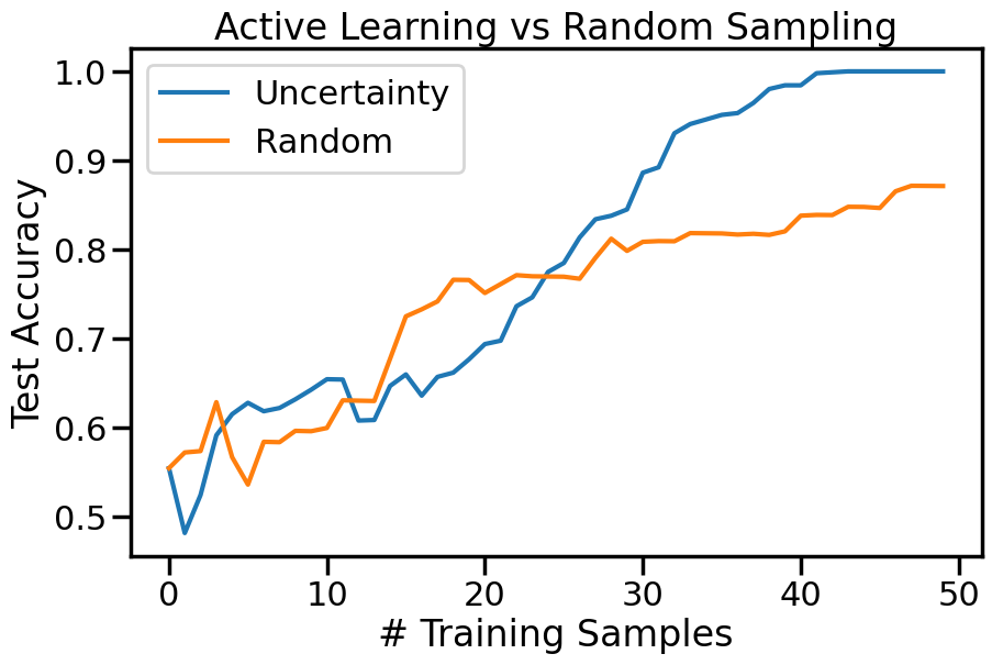
plt.figure(figsize=(10,6))for o in options: # For each sampling option plt.plot(errors[o],label=o)plt.legend()plt.xlabel("# Training Samples")plt.ylabel("Test Accuracy")plt.title("Active Learning vs Random Sampling")plt.show()
TipExperiment: Comparison of Uncertainty Sampling in Classification
You can re-run the above classification experiments with different datasets (e.g., Moons, Circles, Swiss Roll) and varying noise levels. Observe how the performance of Uncertainty Sampling compares to Random Sampling in each case. Consider the following questions:
How are the selected data points distributed using uncertainty sampling? How do they differ from those selected by Random Sampling?
What happens when you increase the noise level on Dataset one (Moons)? How does the relative performance of Uncertainty sampling change as the noise increases?
How does the difference between Uncertainty Sampling and Random Sampling change when we move to more complicated datasets (e.g., Dataset 3 - the swiss roll example?)
How does the comparative behavior of Active Learning change when you change the underlying model (say, in this case, by changing \(\gamma\) – the RBF kernel bandwidth)?
23.6 Semi-Supervised Learning
In addition to Active Learning, we can use Semi-Supervised Learning to leverage the availability of unlabeled data. Semi-Supervised learning works by assigning unlabeled points a label based on nearby supervised data points. Essentially, this uses a subset of labeled data to “imagine” or “propagate” labels to the unlabeled data points. To the extent that nearby points in the input space are likely to share the same label, this can be a powerful way to leverage unlabeled data to improve model performance.
There are several common algorithms for semi-supervised learning, including: - Label Propagation: This algorithm constructs a graph where nodes represent data points and edges represent similarities between points. Labels are then propagated through the graph from labeled to unlabeled nodes based on their connections. - Label Spreading: Similar to label propagation, but it uses a different normalization technique for the graph, which can lead to different propagation dynamics.
In the below example, we will use Label Spreading to demonstrate semi-supervised learning on the same classification problem we saw above. However, despite whatever specific algorithm we might use, the key idea remains the same: we will use the unlabeled data to act as a kind of similiarity measure between points, and then use that similarity measure to decide to what extent certain labeled points should influence the labels of nearby unlabeled points.
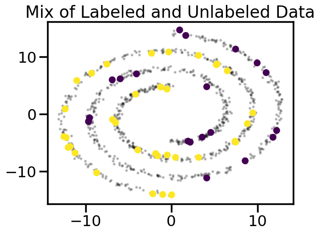
We will start by visualizing a largely unlabeled dataset, but then selecting a few points at random to label. As we can intuitively see below, even with only a few labeled points, we can tell just by looking at the data what labels are likely to occur in some of the unlabeled points:
Code
# Select a small number of starter points:train = train_ind['Random']plt.figure()# Plot in small dots the unlabeled dataplt.scatter(X[~train,0],X[~train,1],c='k',s=5,alpha=0.2)plt.scatter(X[train,0],X[train,1],c=y[train],s=100,lw=0)plt.title("Mix of Labeled and Unlabeled Data")plt.show()
23.6.1 Label Spreading Example
One common algorithm for semi-supervised learning is Label Spreading. This algorithm constructs a graph where nodes represent data points and edges represent similarities between points. Labels are then propagated through the graph from labeled to unlabeled nodes based on what nodes they are connected to.
Specifically, Label Spreading works by first constructing a similarity graph from the data points. The similarity between two points is typically measured using a kernel function, such as the Radial Basis Function (RBF) kernel. Once the graph is constructed, the algorithm iteratively updates the labels of the unlabeled nodes based on the labels of their neighbors, which “closer” neighbors having greater influence. In this way, a label iteratively moves outward from the actual labels through unlabeled nodes. This process continues until convergence, at which point the labels of the unlabeled nodes are assigned based on the propagated labels.
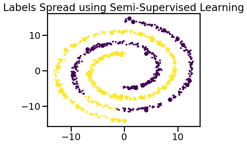
label_prop_model = LabelSpreading(kernel='rbf', gamma=5.0, max_iter=400)labels =-np.ones_like(y)labels[train] = y[train]label_prop_model.fit(X, labels)ll = label_prop_model.transduction_# Plot the resultsplt.figure()plt.scatter(X[:,0],X[:,1],c=ll,lw=0, s=20)plt.scatter(X[train,0],X[train,1],c=y[train],s=100,lw=0)plt.title("Labels Spread using Semi-Supervised Learning")plt.show()
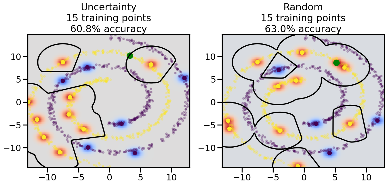
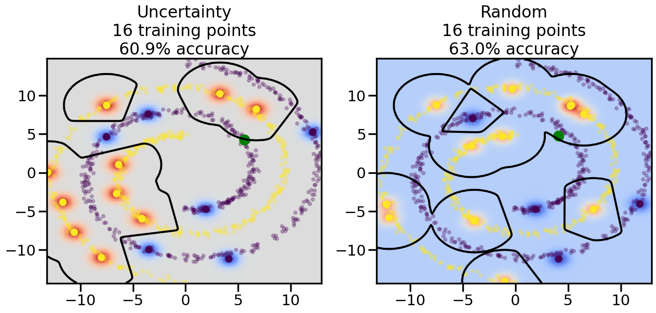
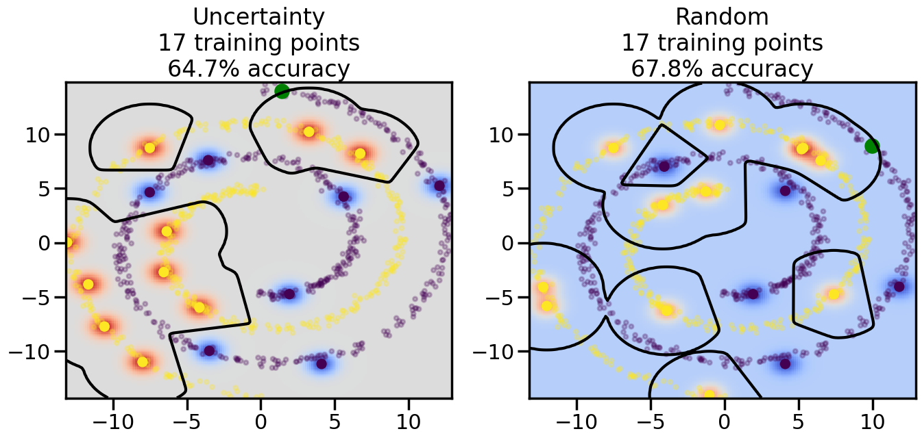
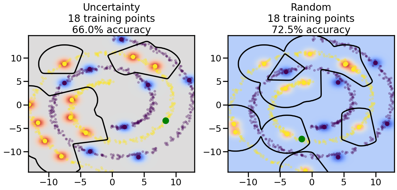
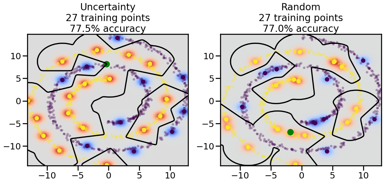
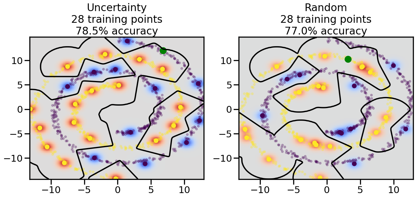
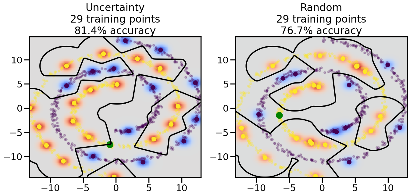
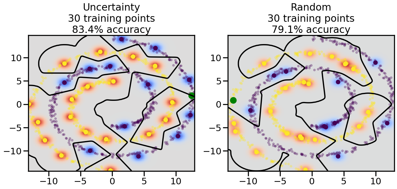
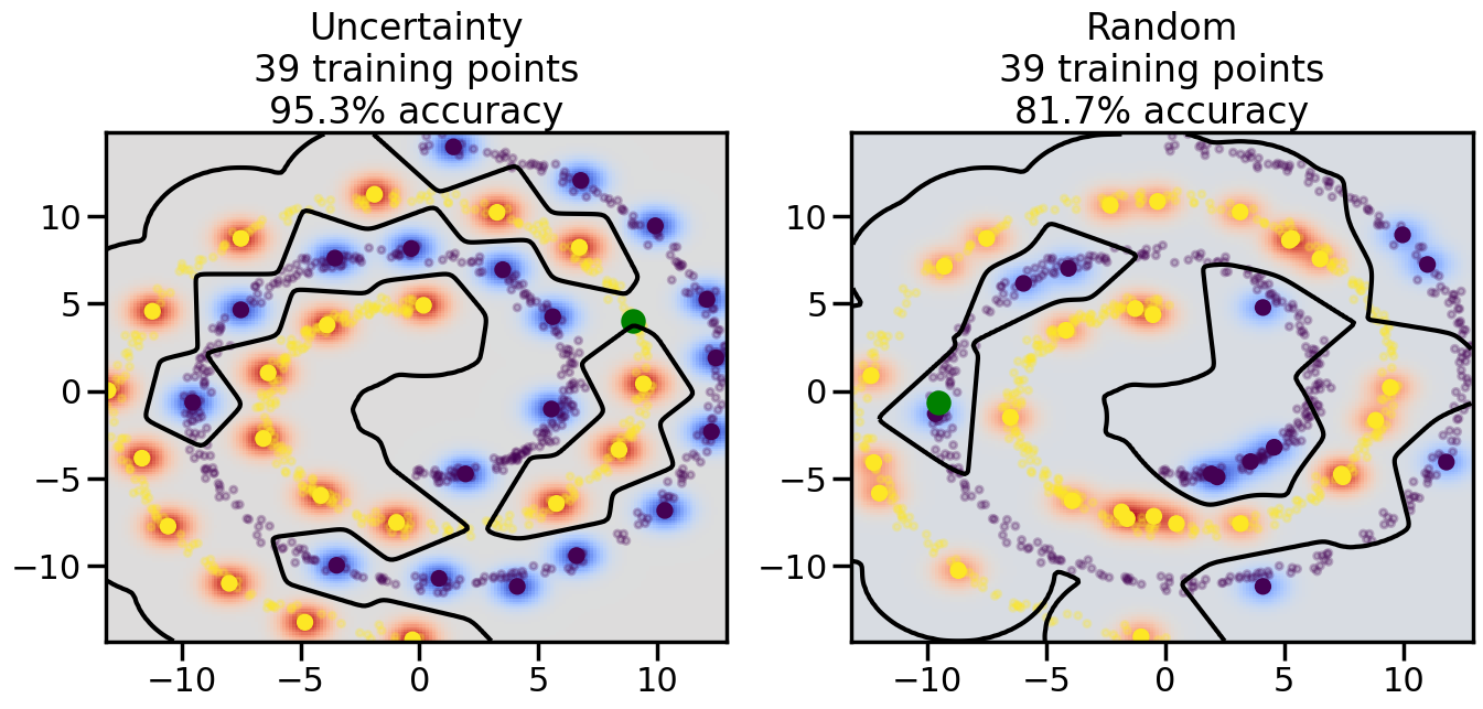
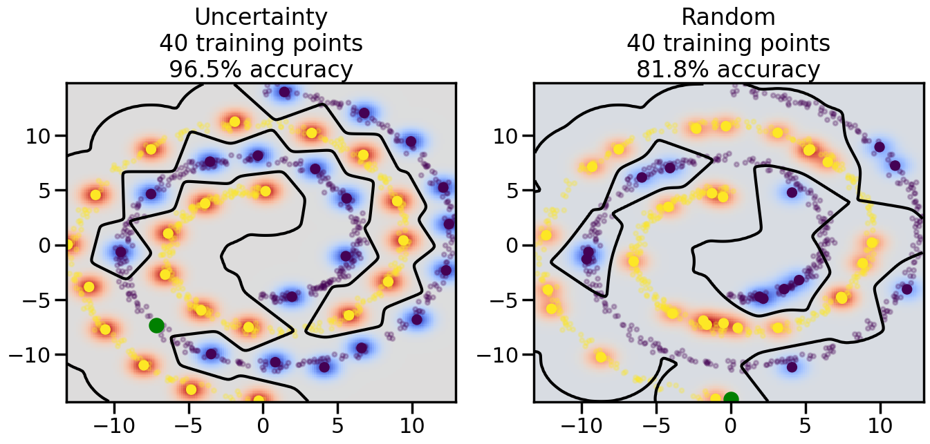
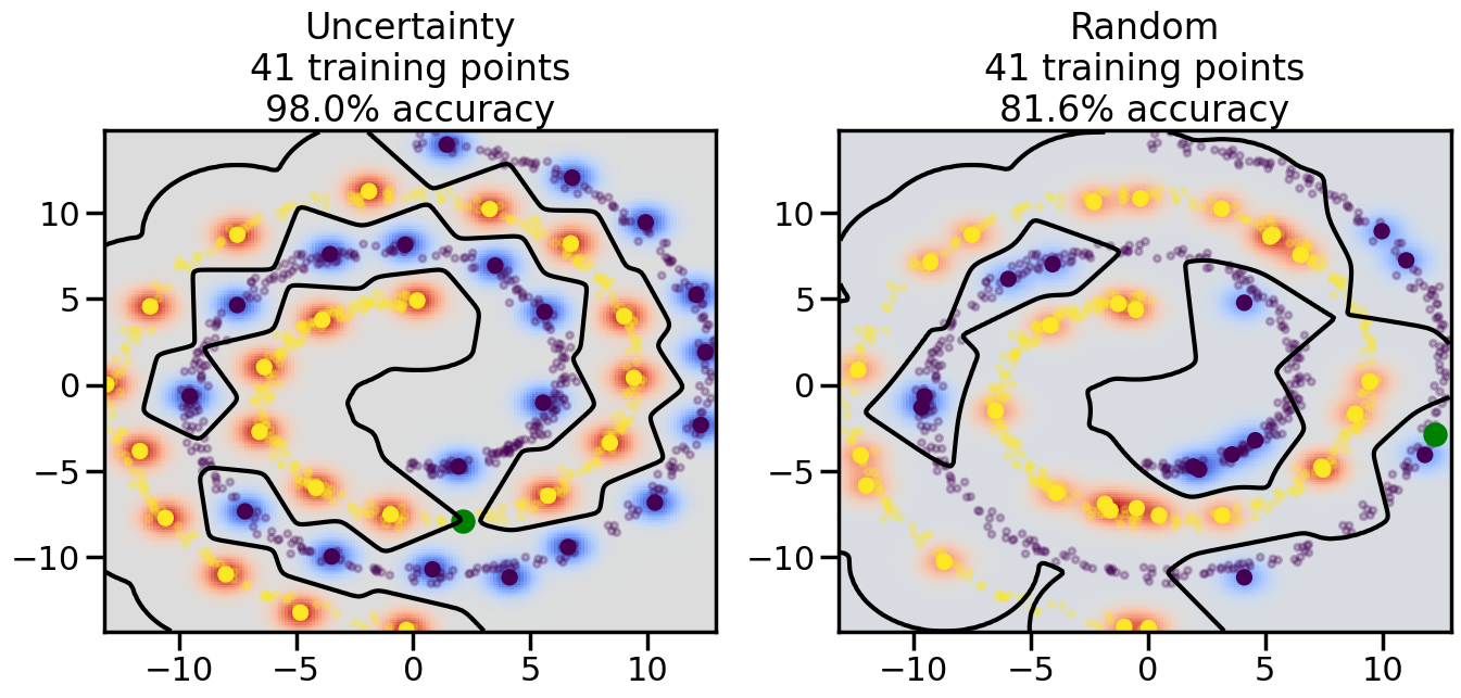
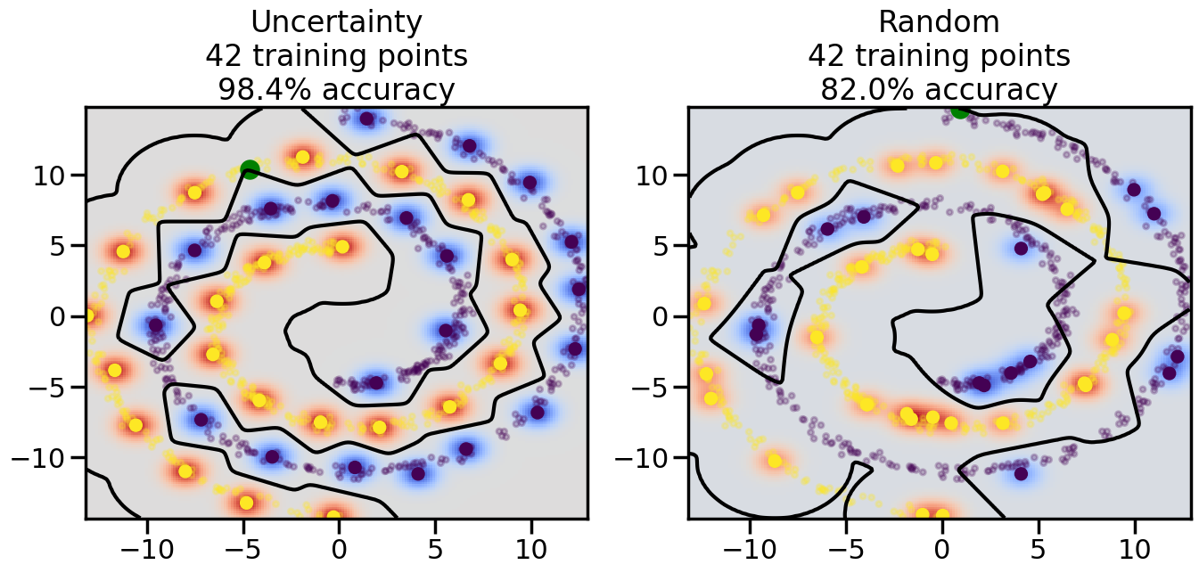
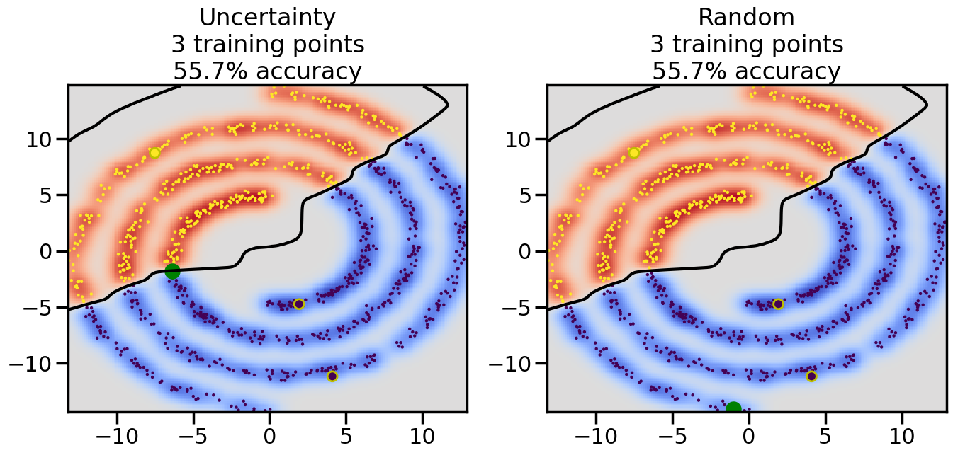
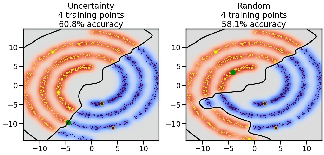
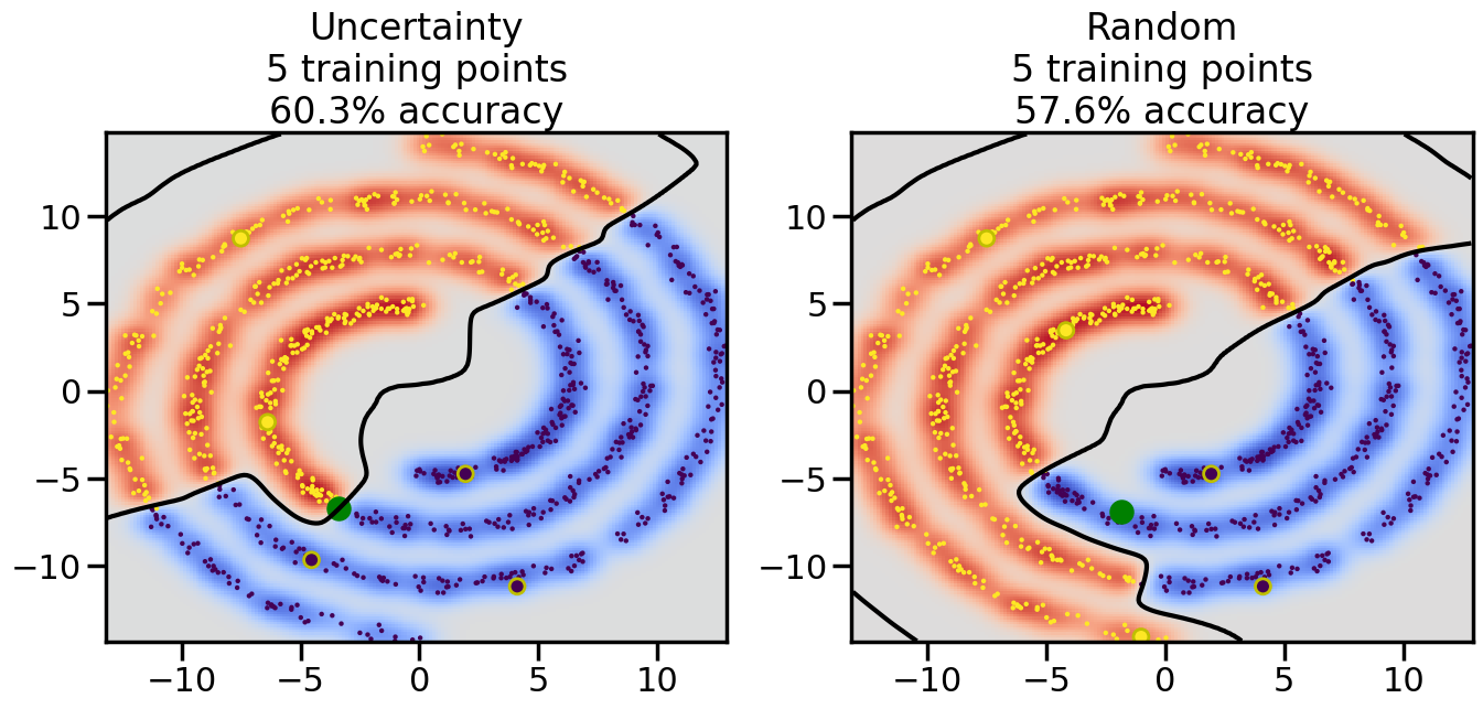
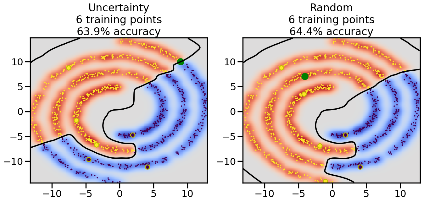
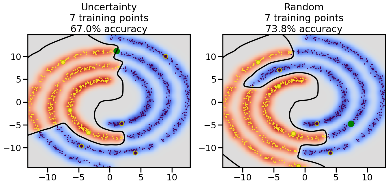
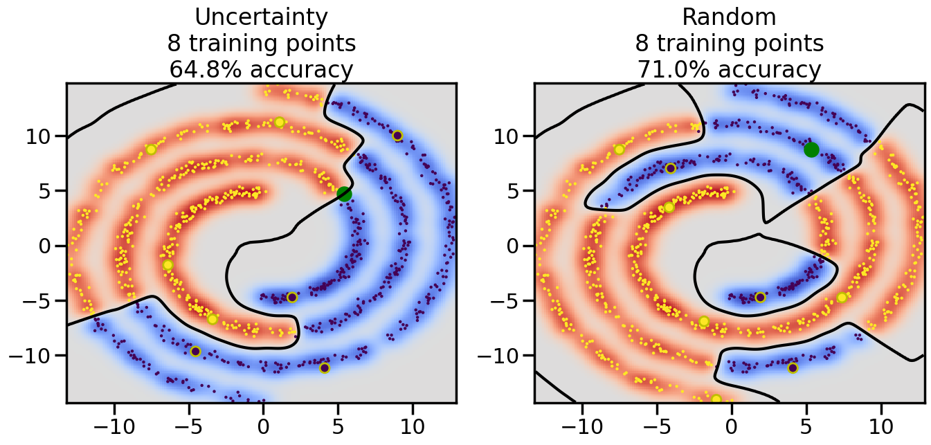
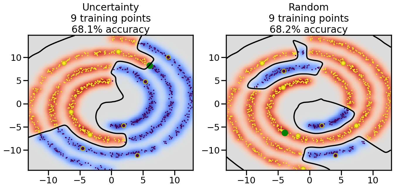
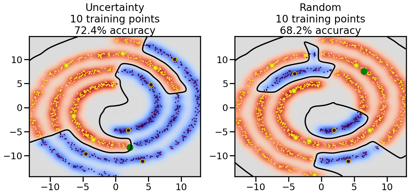
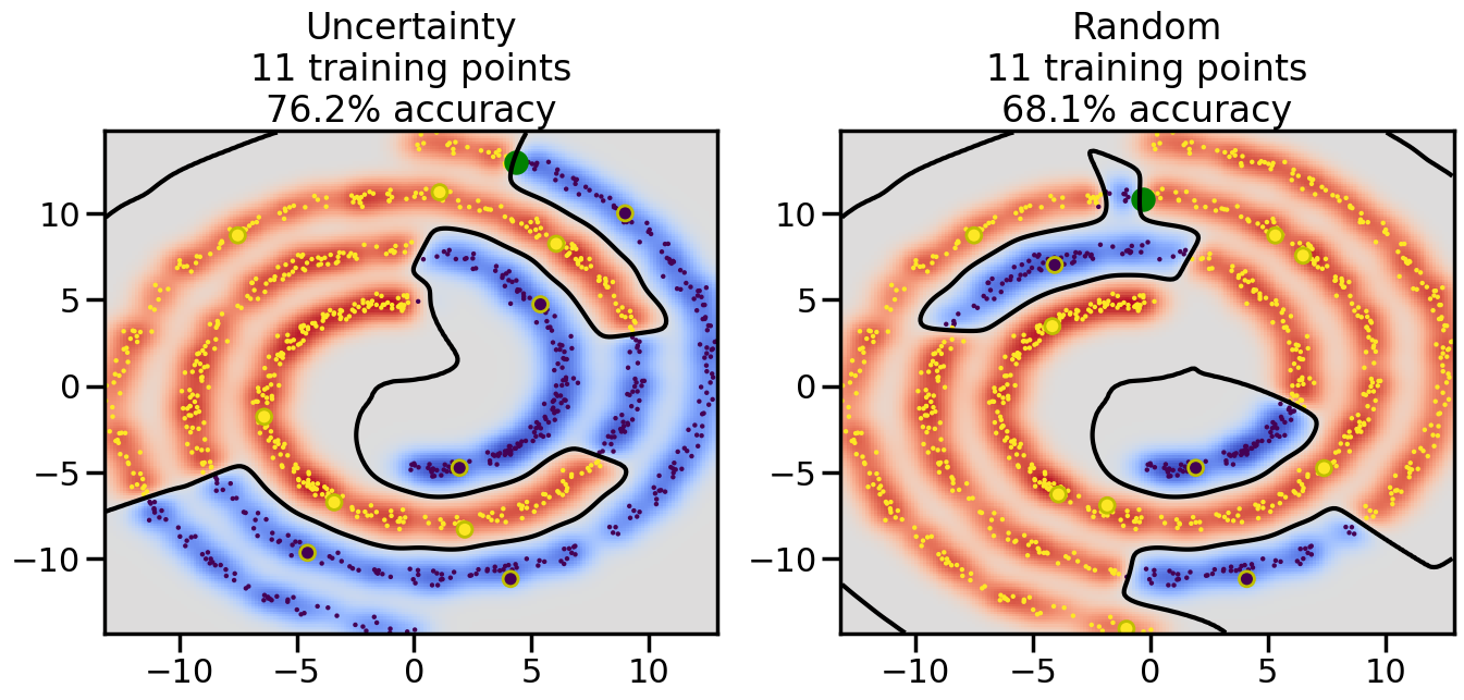
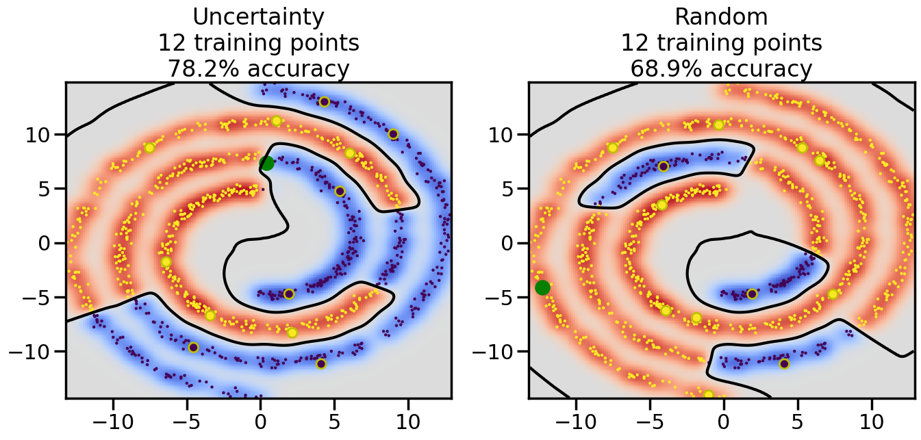
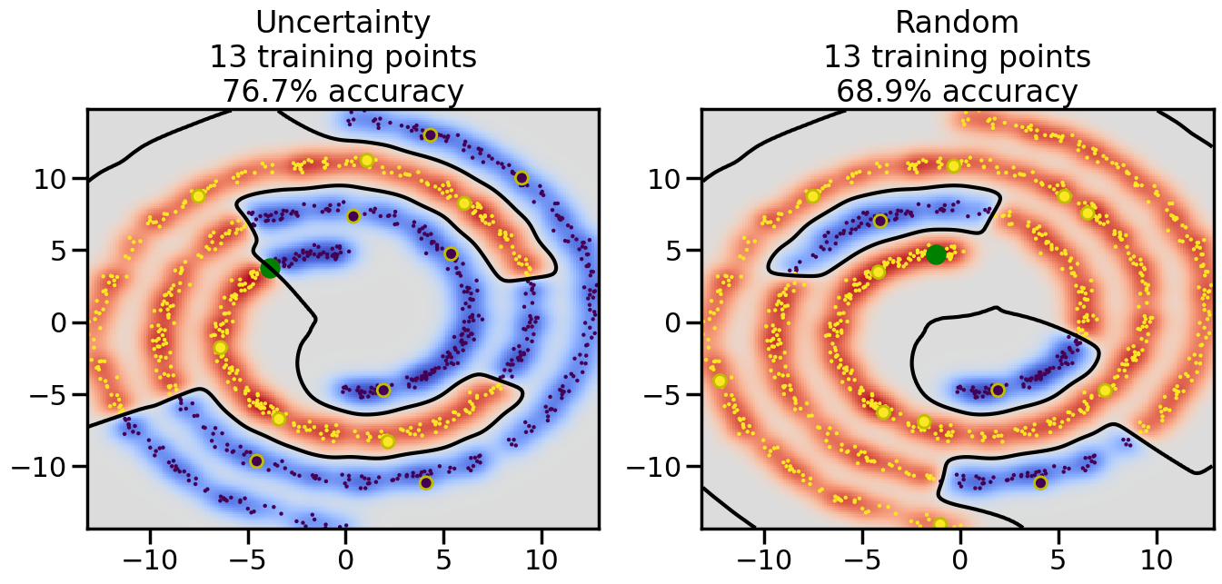
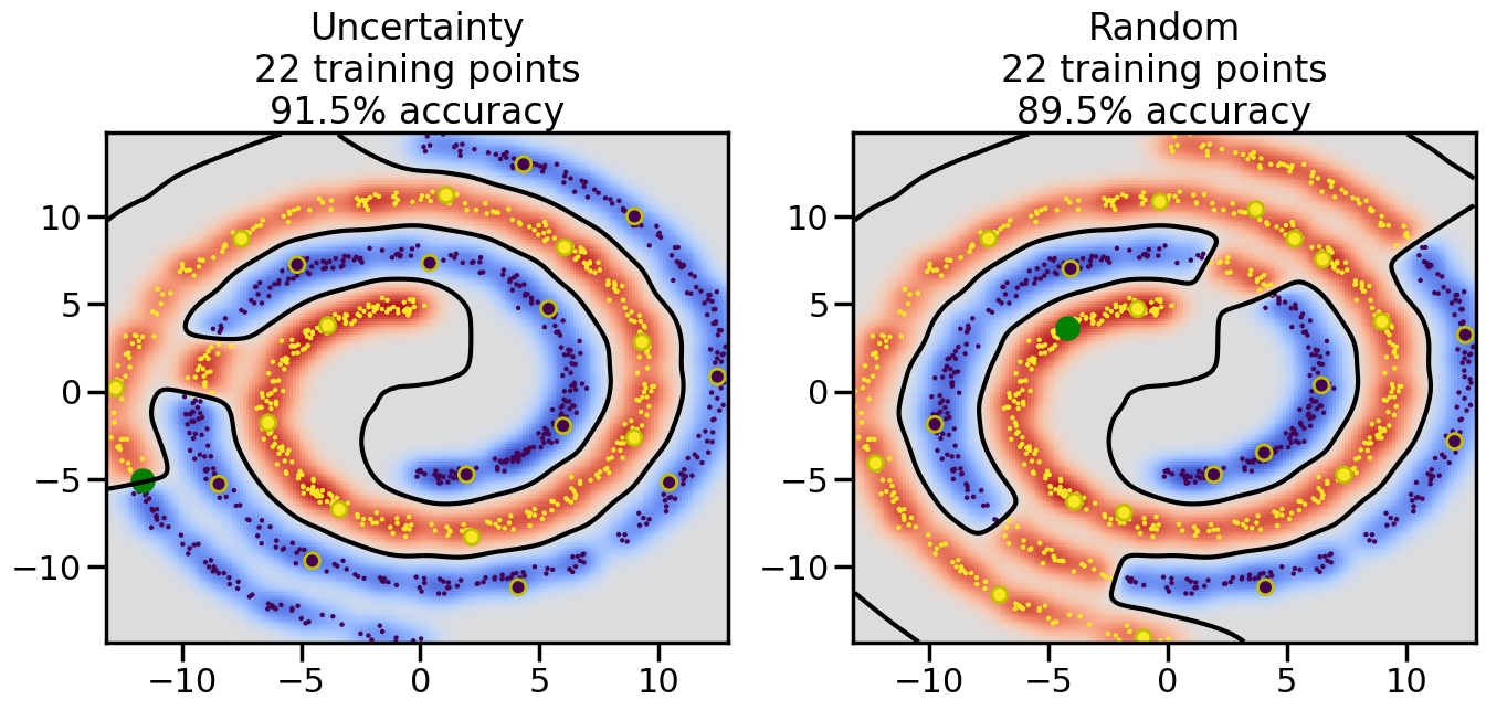
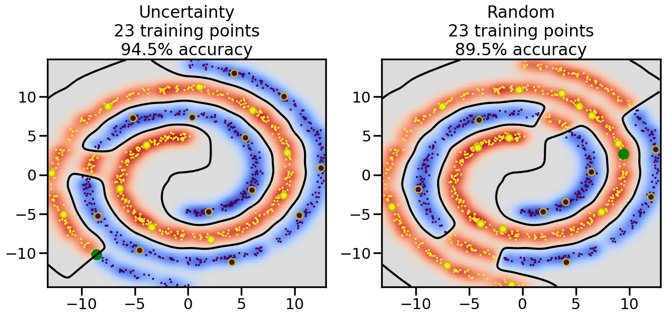
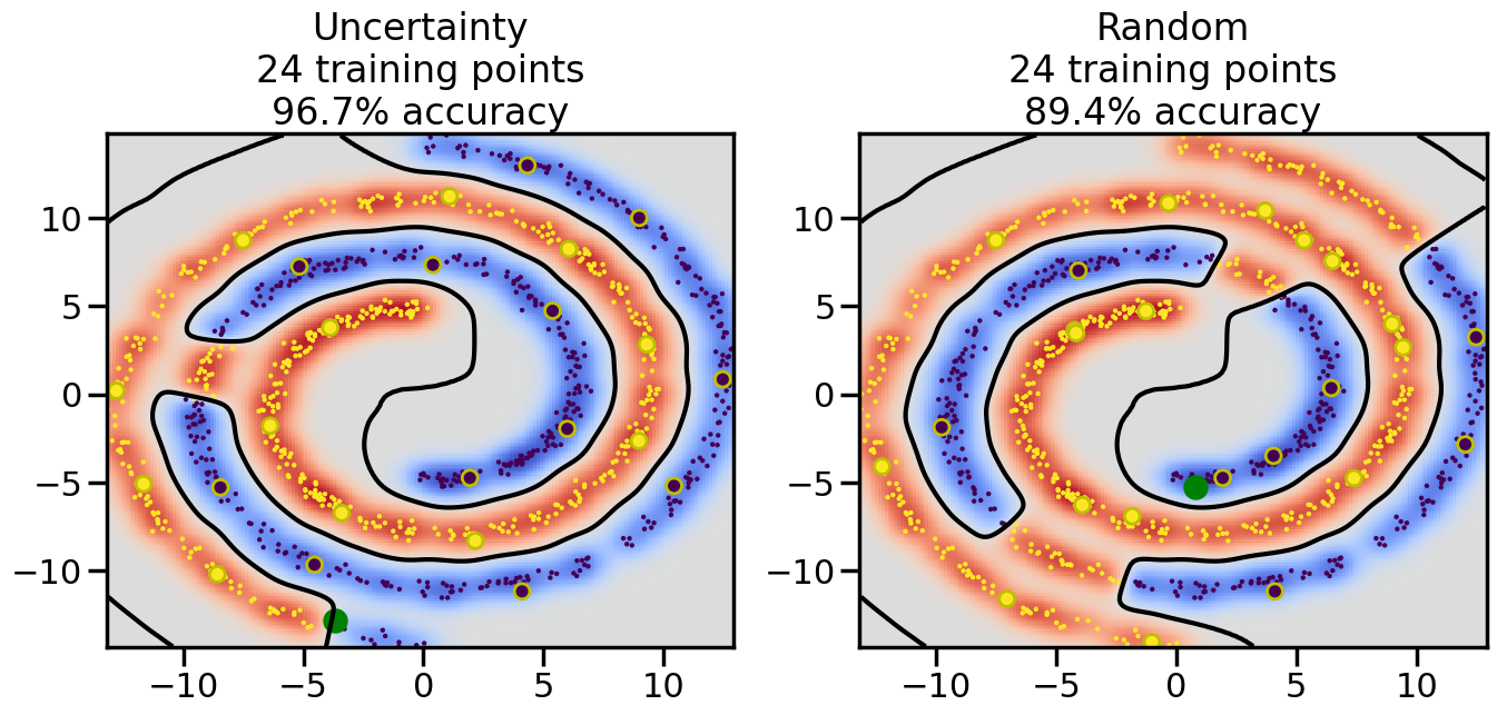
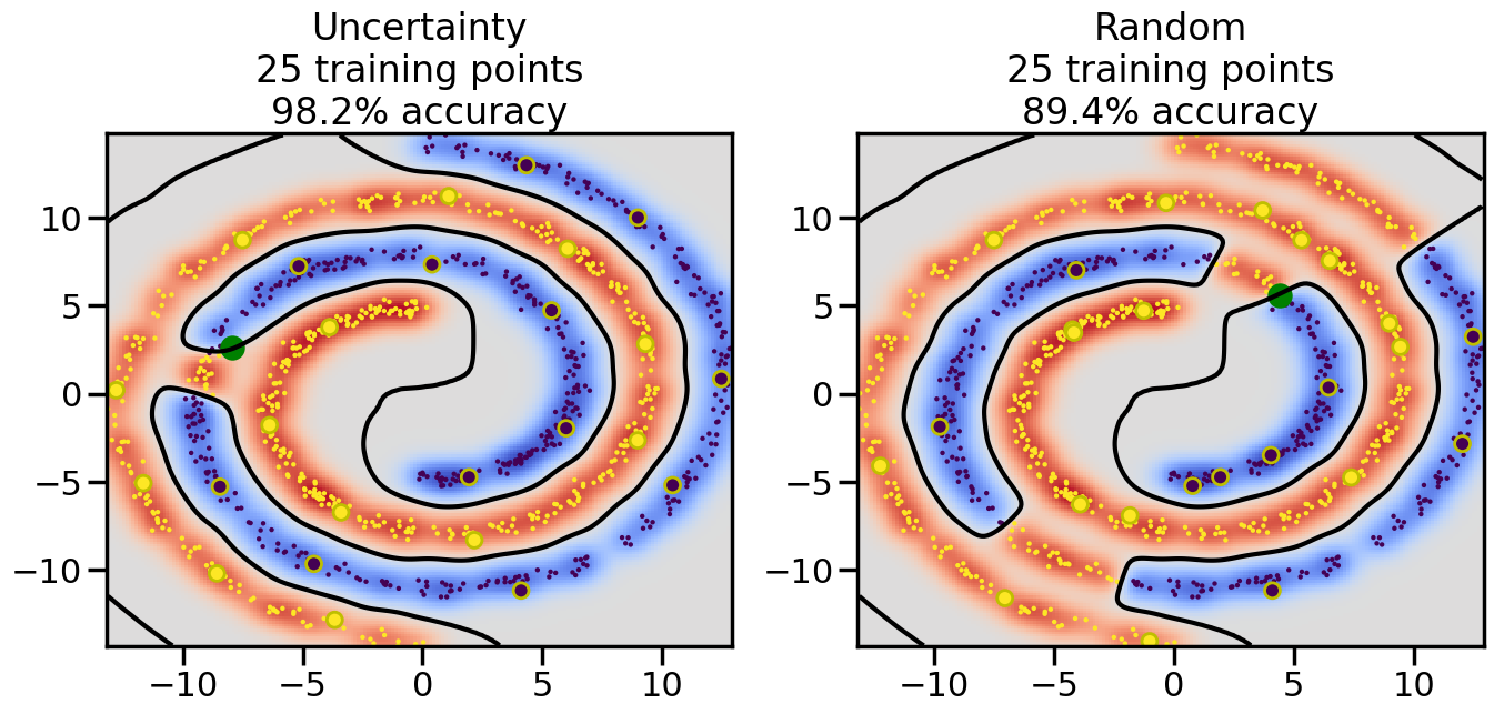
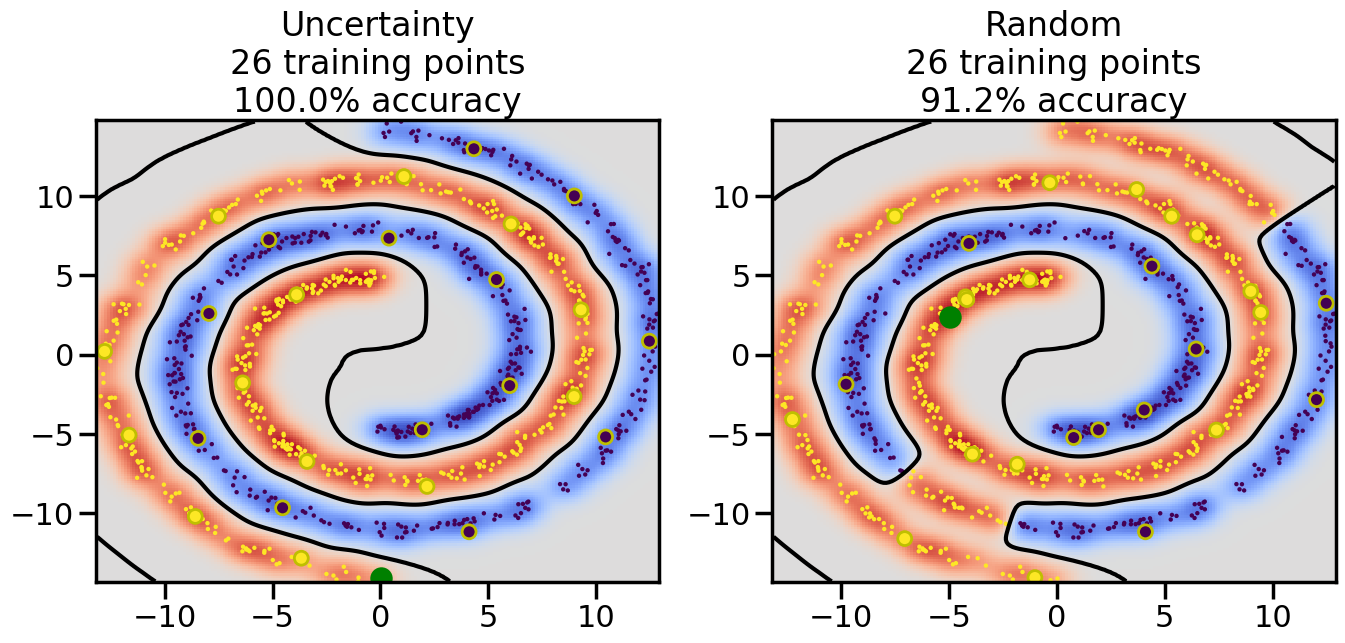
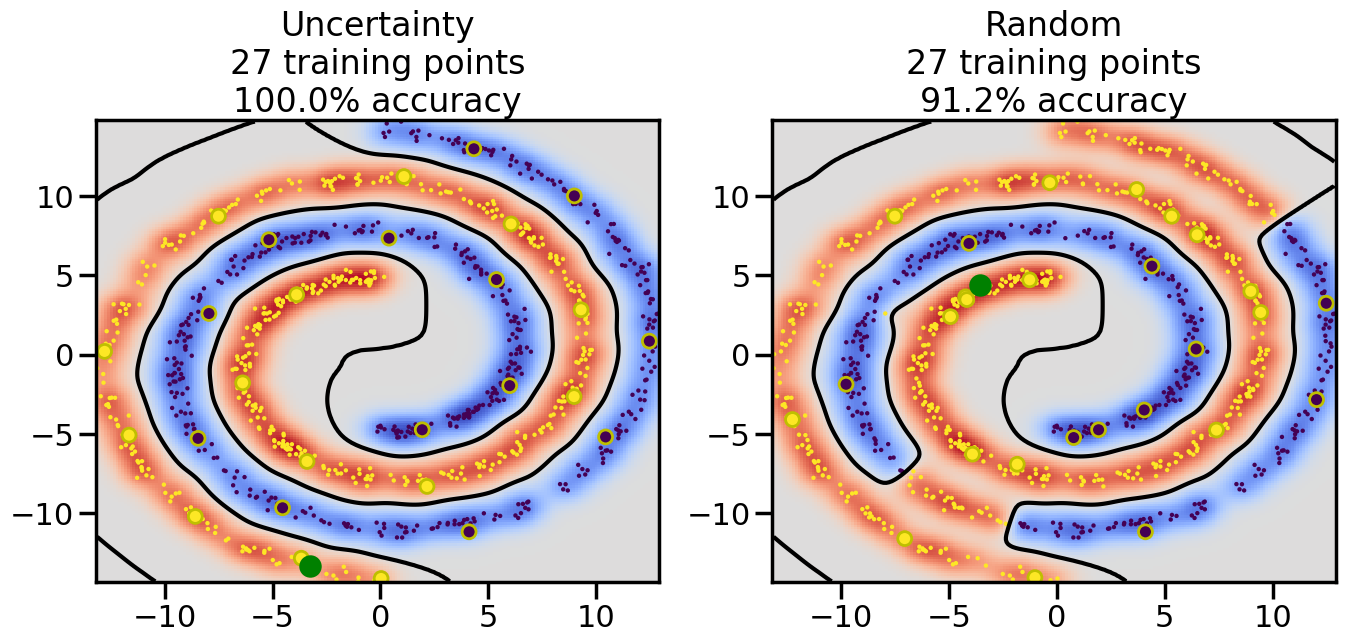
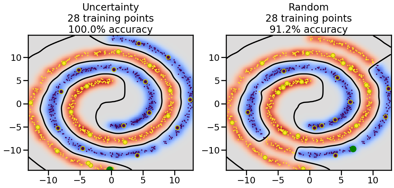
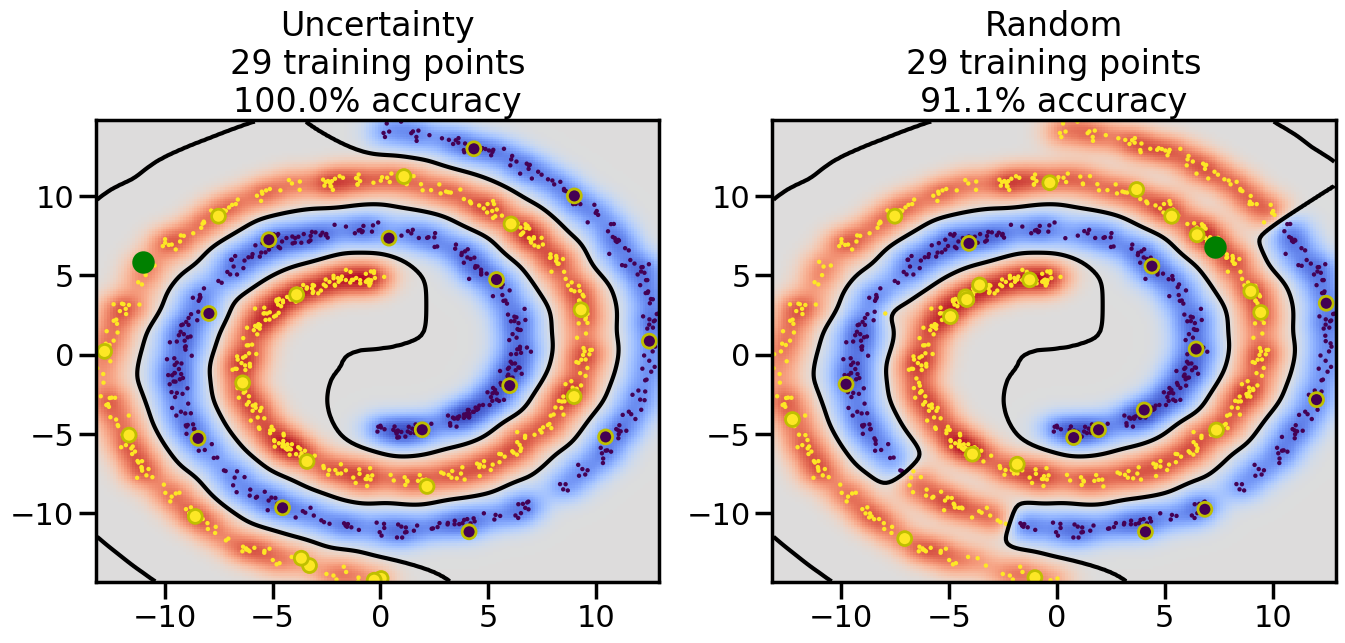
Now we can re-run our above Active Learning experiments, but this time we can also include Label Spreading to “extend the reach” of the samples we collect. Let’s take a look at how incorporating both Active Learning and Semi-Supervised Learning can improve our classification performance compared to using either method alone or neither method at all.
Code
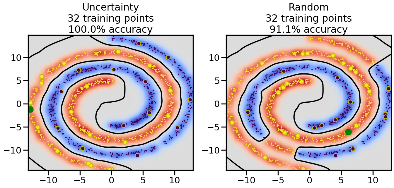
# ------- Try changing the below to modify the classification smoothness -------gamma =0.7# e.g. between 0.1 and 5# --------------------------------------# Reset the random seednp.random.seed(3) # So we all see the same thing# Now, ready to begin learning:train_ind ={'Uncertainty': np.zeros(len(X),dtype=bool),'Random': np.zeros(len(X),dtype=bool)}options = train_ind.keys()possible_points = np.array(list(range(len(X))))# Initializationfor i inrange(3): ind = np.random.choice(possible_points[y==i%2])for o in options: train_ind[o][ind] =True# Classifiersclf = GaussianProcessClassifier(1.0* RBF(length_scale=gamma),optimizer=None)label_prop_model = LabelSpreading(kernel='rbf', gamma=5.0, max_iter=400)# How much data should we collect?num_total_samples =30# Let's store the errors for the models:semi_errors = {'Uncertainty':np.zeros(num_total_samples),'Random':np.zeros(num_total_samples) }for i inrange(num_total_samples):# As i increases, we increase the number of points plt.figure(figsize=(16,6))for j,o inenumerate(options): plt.subplot(1,2,j+1) # Plot intermediate results n_train = np.count_nonzero(train_ind[o])# Do Label Spreading: labels =-np.ones_like(y) labels[train_ind[o]] = y[train_ind[o]] label_prop_model.fit(X, labels) l = label_prop_model.transduction_ clf.fit(X,l) accuracy = clf.score(X[~train_ind[o],:],y[~train_ind[o]])# Plot the decision function x_min = X[:, 0].min() x_max = X[:, 0].max() y_min = X[:, 1].min() y_max = X[:, 1].max() XX, YY = np.mgrid[x_min:x_max:200j, y_min:y_max:200j]#Z = clf.decision_function(np.c_[XX.ravel(), YY.ravel()]) Z = clf.predict_proba(np.c_[XX.ravel(), YY.ravel()])[:,1] -0.5# Put the result into a contour plot Z = Z.reshape(XX.shape) plt.pcolormesh(XX, YY, Z , cmap=plt.get_cmap('coolwarm'),shading='auto') plt.contour(XX, YY, Z, colors=['k', 'k', 'k'], linestyles=['--', '-', '--'], levels=[-.5, 0, .5])# Plot the training points plt.scatter(X[:,0],X[:,1],c=l,lw =0,s=10,alpha=1) plt.scatter(X[train_ind[o],0],X[train_ind[o],1],c=y[train_ind[o]],s=100,lw=2,edgecolor='y')#dists = clf.decision_function(X[~train_ind[o],:]) dists = clf.predict_proba(X[~train_ind[o],:])[:,1] -0.5 dists = np.abs(dists)if o =='Uncertainty': closest_points = np.argwhere(dists == np.amin(dists)).ravel()# Basic Uncertainty sampling---just choose randomly ind = np.random.choice(closest_points) next_point = X[~train_ind[o],:][ind,:].flatten() next_ind = np.argwhere(X == next_point.flatten())[0,0]elif o =='Random': next_ind = np.random.choice(possible_points[~train_ind[o]],1)else:raiseValueError("Invalid option key: {}".format(o)) train_ind[o][next_ind] =True plt.scatter(X[next_ind,0],X[next_ind,1],c='g',s=200) semi_errors[o][i]=accuracy plt.title("%s\n%d training points\n%.1f%% accuracy"%(o,n_train,accuracy*100)) plt.show()
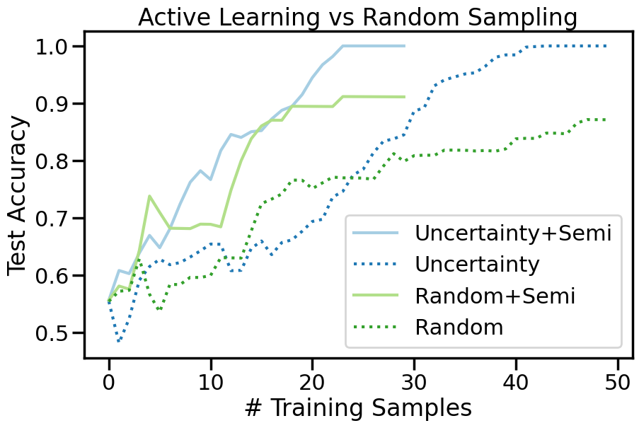
We can alsop compare the accuracy versus sample curve from before and after Semi-Supervised learning to see how much of a difference it makes:
Code
plt.figure(figsize=(10,6))ax = plt.axes()ax.set_prop_cycle('color',[plt.cm.Paired(i) for i in np.linspace(0, 1, 12)])for o in options: # For each sampling option plt.plot(semi_errors[o],label=o+'+Semi') plt.plot(errors[o],':',label=o)plt.legend()plt.xlabel("# Training Samples")plt.ylabel("Test Accuracy")plt.title("Active Learning vs Random Sampling")plt.show()
TipExperiment: When and Where does Semi-Supervised Learning Help?
Compare and constrast your results from the above Active Learning experiments with those using Semi-Supervised Learning and consider the following questions:
How does Semi-Supervised learning (using both Uncertainty and Random Sampling) compare to the non-semi-supervised cases you saw above?
In what ways does the use of Uncertainty Sampling + Semi-Supervised sampling change the location of sampled data points, compared to uncertainy sampling by itself?
How does Active + Semi-Supervised learning perform on Dataset 3, relative to just Active Learning by itself on Dataset 3? Why does it perform so differently?
Is Active + Semi-Supervised learning always better than either approach by itself? What happens in Dataset 4 (Moons + Gaussian)?
23.7 Summary
In this chapter, we explored the concepts of Active Learning and Semi-Supervised Learning, two powerful techniques for making the most of limited labeled data. We discussed various strategies for selecting informative data points in Active Learning, with a focus on Uncertainty Sampling due to its simplicity and effectiveness. We also examined how Semi-Supervised Learning can leverage unlabeled data to improve model performance through techniques like Label Spreading.
Overall, both Active Learning and Semi-Supervised Learning can significantly enhance model performance in scenarios where labeled data is scarce or expensive to obtain. By intelligently selecting data points to label and utilizing unlabeled data, these techniques allow us to build more accurate and robust models with fewer resources. However, we also saw a few downsides. Notably, both Active Learning and Semi-Supervised learning can become overly confident, leading the model to ignore sampling regions where it is particularly confident, even if those regions are actually incorrect. Thus, an over-reliance on only gathering samples using Active Learning could bias the model away from sampling regions that might, in the long run, be more informative.